
If your formula is starting to repeat the same subexpression two or three times, or is getting so long that you’ve lost track of what each piece means, the LET function in Google Sheets is what you need.
LET lets you name a calculation, then reuse that name as if it were a variable. The result is a formula that reads top to bottom and computes each part only once. In this article, I’ll walk through five examples showing where LET earns its place.
LET Function Syntax in Google Sheets
Here is how the LET function is written:
=LET(name1, value1, [name2, value2, ...], expression)
- name1, name2, … are the variable names you choose.
- value1, value2, … are the expressions or cell references those names point to.
- expression is the final calculation that uses the names. It must be the last argument.
You can declare as many name-value pairs as you need. The last argument is always the expression that produces the result.
When to Use LET Function
- Stop repeating the same subexpression in a long formula.
- Name intermediate steps so the formula reads like a recipe instead of a wall of parentheses.
- Compute an expensive piece once and reuse it without recalculating.
- Make tiered thresholds or constants visible by name inside the formula.
- Pair LET with IF or other functions to clean up nested logic.
Example 1: Avoid Repeating A Subexpression With LET
Let’s start with the simplest case, naming a value so you can use it twice.
Below is the dataset, with the product name in column A, the base price in column B, the discount in column C, and an empty Final Price column D, across rows 2 to 6.
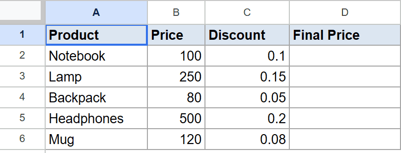
You want the final price as the taxed price minus the discount on that taxed price. The taxed price is B2*1.1, and without LET you’d type that twice.
Here is the formula:
=LET(taxed, B2*1.1, taxed - taxed*C2)
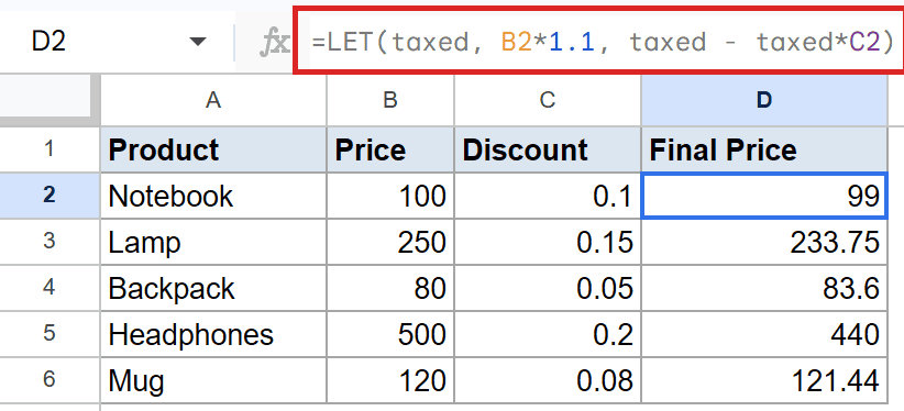
How this formula works:
taxedis the name.B2*1.1is its value. So for row 2, taxed becomes 110.- The final expression
taxed - taxed*C2uses the name twice without recomputingB2*1.1. - For row 2 with a 10 percent discount on 110, the result is 99.
If you had to repeat B2*1.1 - B2*1.1*C2 and then change the tax rate later, you’d have to remember to update both copies. With LET, the rate lives in one place.
Example 2: Chain A Multi-Step Calculation
LET really shines when you have several intermediate steps.
Below is the dataset, with Customer in column A, Units in B, Price in C, Tax Rate in D, Discount in E, and an empty Final column F, across rows 2 to 6.
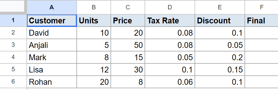
You want a final amount that goes through revenue, then tax, then total before discount, then a final discounted total. Without LET, you’d be nesting everything in one giant expression.
Here is the formula:
=LET(revenue, B2*C2, tax, revenue*D2, after_tax, revenue+tax, after_tax*(1-E2))
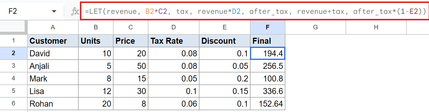
How this formula works:
revenueis units times price.taxis revenue times the tax rate, and it reuses therevenuename from the previous step.after_taxis revenue plus tax, the pre-discount total.- The final expression multiplies
after_taxby one minus the discount.
For the first row, that flow is 200 revenue, 16 tax, 216 after tax, and 194.4 final. The formula reads like a flowchart.
Pro Tip: Each name can reference any name declared before it. So `tax` can use `revenue`, and `after_tax` can use both. Order matters, you can’t reference a name above where it’s defined.
Example 3: Wrap Tiered Bonus Thresholds Once
A nested IF with hard-coded thresholds is a classic place to use LET.
Below is the dataset, with Salesperson in column A, Sales in column B, and an empty Bonus column C, across rows 2 to 6.
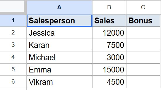
You want a bonus of 10 percent for sales of 10,000 or more, 5 percent for sales of 5,000 or more, and 2 percent below that. Hard-coding 10000 and 5000 into a nested IF buries those thresholds in the middle of the formula.
Here is the formula:
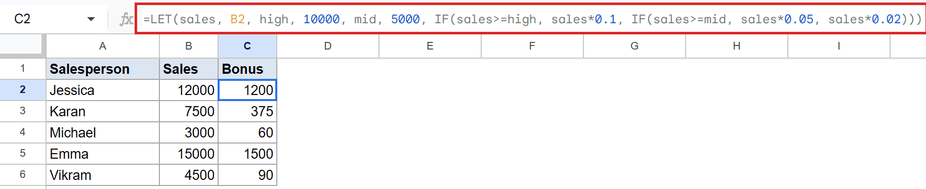
=LET(sales, B2, high, 10000, mid, 5000, IF(sales>=high, sales*0.1, IF(sales>=mid, sales*0.05, sales*0.02)))
How this formula works:
salesnamesB2so the rest of the formula reads with English instead of cell refs.highandmidname the two threshold values at the top of the formula, easy to spot and change.- The nested IF uses those names: if sales is above the high threshold, apply 10 percent, otherwise check the mid threshold, otherwise 2 percent.
Row 2 with sales of 12,000 lands in the top tier and the result is 1200. Row 3 at 7,500 lands in the mid tier and produces 375. Row 4 at 3,000 drops to the bottom tier.
When you decide next quarter to push the high threshold up to 12,000, you change one number at the top of the formula instead of hunting through the nested IF.
Example 4: Reuse A VLOOKUP Result Twice
Lookups are a great spot for LET, since you usually want to use the looked-up value more than once.
Below is the dataset, with a small price table in columns A and B, then customer orders in columns D through F, and an empty Total column G, across rows 2 to 6.
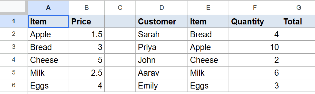
You want the total for each order as the looked-up price times quantity times 1.08 for tax. Without LET, you’d write the VLOOKUP twice if the formula needed the price more than once.
Here is the formula:
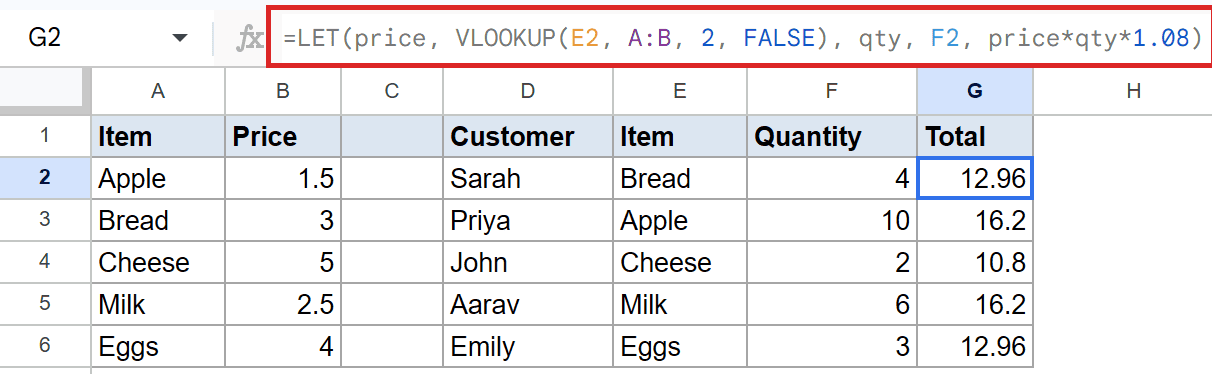
=LET(price, VLOOKUP(E2, A:B, 2, FALSE), qty, F2, price*qty*1.08)
How this formula works:
priceruns the VLOOKUP once and stores the looked-up price.qtynames the quantity from column F.- The final expression multiplies
pricebyqtyand by 1.08 for tax.
Row 2 looks up Bread, finds a price of 3.00, multiplies by 4 units and 1.08 tax, and the answer is 12.96. Beyond readability, LET keeps the VLOOKUP from running twice if you ever extend the formula to also display the price alongside the total.
Example 5: Adjust A Score Halfway To The Max
LET works just as happily with ranges as it does with single cells.
Below is the dataset, with three test scores in columns A, B, and C, and an empty Adjusted column D, across rows 2 to 6.
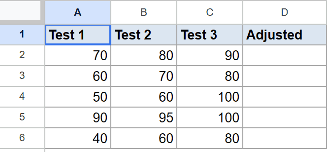
You want an adjusted score that’s the row’s average pushed halfway toward that row’s max.
Here is the formula:
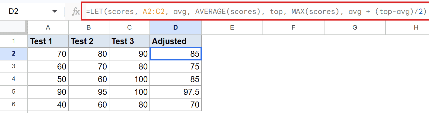
=LET(scores, A2:C2, avg, AVERAGE(scores), top, MAX(scores), avg + (top-avg)/2)
How this formula works:
scoresnames the row rangeA2:C2. The name now stands for that whole range.avgruns AVERAGE on the named range.topruns MAX on the same named range.- The final expression takes the average and adds half the distance from average to max.
Row 2 has scores 70, 80, 90. The average is 80, the max is 90, halfway between is 85. The formula produces 85 for that row.
Naming the range once means you only type A2:C2 in one place. If the columns shift later, you update one reference and the rest of the formula stays untouched.
Pro Tip: LET pairs naturally with LAMBDA. You can wrap a LET formula in a LAMBDA to turn it into a reusable named function via Sheets’ Named Functions feature.
Tips & Common Mistakes
- Variable names can’t collide with built-in function names. Don’t name a variable
MAX,SUM,IF, or any other function. Sheets will throw a parse error. Pick descriptive names liketop,total,flaginstead. - Name-value pairs MUST come before the final expression. LET expects pairs first, then exactly one final expression as the last argument. If you forget the final expression, or sneak another pair after it, the formula breaks. The last argument is always the answer.
- Long LET chains can be harder to debug than flat formulas. When the shape of the calculation changes, you have to walk every name to see what’s still valid. If a formula has two or three steps, LET helps. If it has a dozen, consider breaking it into helper columns instead.
LET is one of those functions that quietly upgrades the rest of your spreadsheet work. Once you start naming intermediate steps, your formulas become things you can actually read six months later.
Reach for it the moment you catch yourself typing the same expression twice, or losing your place inside a nested formula.
List of All Google Sheets Functions
Related Google Sheets Functions / Articles: