DATEVALUE Function in Google Sheets

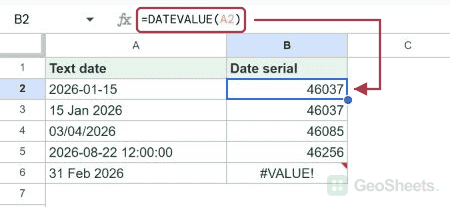
If you want to convert a date written as text into a real date that Google Sheets can sort, filter, and do math with, the DATEVALUE function is the tool for the job. It takes a date string and returns the underlying date serial number.

In this article, I’ll show you how DATEVALUE handles ISO dates, long-form dates, and date strings with a time component. I’ll also cover how to compose a date from separate columns and how to compute the days between two dates.

DATEVALUE Function Syntax in Google Sheets

The DATEVALUE function converts a date string into a date serial number.

=DATEVALUE(date_string)
  • date_string is the text you want to convert. It can be a literal string in quotes or a cell reference like A2. Common formats include 2026-01-15, January 15 2026, and 15-Jan-2026.

DATEVALUE returns a serial number, not a formatted date. The cell shows something like 46037 by default. To see it as a readable date, highlight the column, open the Format menu, pick Number, then Date.

When to Use DATEVALUE Function

  • Convert dates pasted in as text into real dates you can sort and filter.
  • Turn a Year, Month, and Day spread across three columns into a single date value.
  • Strip the time component off a date with time string and keep just the date.
  • Compute the number of days between two date strings without rebuilding the data.
  • Feed a date string from a CSV import into formulas that expect a real date.

Example 1: Convert ISO Format Date Strings to Serial Numbers

Let’s start with the simplest case, an ISO date written as YYYY-MM-DD.

Below is the dataset. Column A has five date strings in ISO format.

Google Sheets: Column A titled "Date String" contains five YYYY-MM-DD date examples.

I want to convert each string into a real date in column B.

Here is the formula:

=DATEVALUE(A2)
Google Sheets: Formula `=DATEVALUE(A2)` converts "2026-01-15" to serial 46037 in cell B2.

DATEVALUE reads the text in column A and outputs the matching date serial. The first row, 2026-01-15, becomes 46037. The second row, 2026-03-22, becomes 46103.

The cell shows a raw number because DATEVALUE returns the underlying serial. Highlight column B, open the Format menu, pick Number, then Date, and each serial flips to a readable date.

Pro Tip: If you’d rather use one formula instead of filling down, wrap DATEVALUE in ARRAYFORMULA, like this: =ARRAYFORMULA(DATEVALUE(A2:A6)). Same result, one cell.

Example 2: Compose a Date From Year, Month, and Day Columns

A lot of exported data shows the year, month, and day in separate columns. DATEVALUE can stitch them back together when paired with string concatenation.

Below is the dataset. Column A has the year, column B has the month, and column C has the day.

Google Sheets example 2 dataset: Year, Month, Day columns for DATEVALUE tutorial.

I want to combine the three pieces into one date in column D.

Here is the formula:

=DATEVALUE(A2&"-"&B2&"-"&C2)
Google Sheets: D2 formula =DATEVALUE(A2&"-"&B2&"-"&C2) returns serial date 46037.

The & operator glues the three cells together with hyphens. The combined string in row 2 reads 2026-1-15, and DATEVALUE turns it into the serial 46037.

Row 3 builds 2025-4-30, landing on 45777. Row 4 builds 2024-11-3, landing on 45599. Format column D as a date to see each result in calendar form.

Example 3: Convert Long Form Dates With Month Names

DATEVALUE also parses long-form dates like January 15, 2026. This is useful when you copy dates straight from prose or from an email.

Below is the dataset. Column A has five long-form date strings.

Google Sheet with 'Date String' header and five example date strings.

I want the matching date serial in column B.

Here is the formula:

=DATEVALUE(A2)
Google Sheets showing DATEVALUE(A2) formula converting "January 15, 2026" to 46037 in B2.

DATEVALUE handles the comma and the month name without any extra cleanup. January 15, 2026 becomes the serial 46037. October 31, 2024 becomes 45596.

The same rule applies. Format column B as a date if you want each number to show as a readable date instead of a raw serial.

Example 4: Strip the Time Off a Date With Time String

When a string carries a time component like 2026-01-15 09:30:00, DATEVALUE keeps the date part and drops the time. The result is always a whole-number serial.

Below is the dataset. Column A has five date-and-time strings.

Google Sheet with a 'Date String' column displaying five date-time values.

I want just the date as a serial in column B, without the time.

Here is the formula:

=DATEVALUE(A2)
Google Sheets: DATEVALUE(A2) converts a date string to serial number 46037 in B2.

The first row, 2026-01-15 09:30:00, becomes 46037. The time 09:30:00 is ignored. The third row, 2026-08-22 12:00:00, becomes 46256. The 12:00 noon is gone too.

This trick is handy when you have timestamped data and you want to group rows by day. Run each timestamp through DATEVALUE and now every row from the same calendar day shares one serial number.

Pro Tip: If your input is already a real datetime value, not a text string, use INT(A2) instead. INT chops off the fractional part the same way and works on actual dates. DATEVALUE only takes text input.

Example 5: Days Between Two Dates Using DATEVALUE

Once you have date serials, you can subtract them to find the gap in days. DATEVALUE makes this work even when the input is text.

Below is the dataset. Column A has a start date and column B has an end date, both as text in D-Mon-YYYY format.

Google Sheets dataset with 'Start' and 'End' date string columns.

I want the number of days between the two dates in column C.

Here is the formula:

=DATEVALUE(B2)-DATEVALUE(A2)
Google Sheets: DATEVALUE formula `=DATEVALUE(B2)-DATEVALUE(A2)` in C2 calculates 14.

DATEVALUE converts each string to a serial, then the subtraction gives the day count. The first row, 1-Jan-2026 to 15-Jan-2026, returns 14. The second row, 25-Dec-2025 to 10-Jan-2026, returns 16. Both March and June span 30 days, and the last row gives 6.

Because the result is a count, format column C as a plain number, not a date. Date formatting on 14 would show January 13, 1900, which isn’t what you want.

Since the dates are already numbers under the hood, you can also feed these serials into other functions like SUMIFS for date-range totals.

Tips & Common Mistakes

  • Format the result column as a date. DATEVALUE returns a serial number by default, so the cell shows a raw integer. Highlight the column, open Format, pick Number, then Date, and each serial becomes a readable date.
  • Input must be text, not a real date. DATEVALUE expects a string. If you pass a real date cell, it throws a #VALUE! error. Use INT instead for real datetime inputs.
  • Locale affects parsing. A string like 03/04/2026 reads as March 4 in a US locale and April 3 in a UK locale. If your spreadsheet locale doesn’t match your data, change it under File then Settings, or use unambiguous formats like 2026-03-04.

DATEVALUE is the bridge between text dates and real dates in Google Sheets. Once a string passes through it, the result behaves like any other date you’d type by hand.

You’ve now seen it parsing ISO dates, composing dates from separate columns, handling long-form text, stripping time components, and computing day gaps. Format the result as a date when you want to read it, and as a number when the result is a day count.

List of All Google Sheets Functions

Related Google Sheets Functions / Articles: