NOT Function in Google Sheets

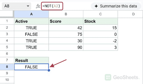
If you need to flip a TRUE to a FALSE or check that something is not the case, the NOT function in Google Sheets handles it in one call. You pass it a logical value or condition, and it returns the opposite.

I’ll walk through five examples, covering plain booleans, inverted comparisons, NOT inside IF, NOT wrapped around AND, and a text exclusion.

NOT Function Syntax in Google Sheets

NOT takes a logical value and returns its opposite.

=NOT(logical_expression)

• logical_expression is the value or condition you want to flip. It can be TRUE, FALSE, a comparison like A2>50, or any expression that evaluates to TRUE or FALSE.

When to Use NOT Function

• Flip a column of TRUE and FALSE values into their opposites for an inverted view.
• Invert a comparison when the negative case is easier to write than the positive one.
• Pair with IF to return one label when a condition fails and another when it passes.
• Combine with AND or OR to flag rows that miss at least one requirement.
• Match every value except one specific text label or number.

Example 1: Flip TRUE and FALSE Values

Let’s start with the simplest job, flipping a column of booleans.

Below is the dataset. Column A has five TRUE and FALSE values marking which accounts are active.

I want column B to show the opposite, an Inactive flag for each row.

Here is the formula:

=NOT(A2)

NOT looks at each value in column A and returns its opposite in column B. The TRUE rows become FALSE and the FALSE rows become TRUE, so the Inactive column reads FALSE, TRUE, FALSE, FALSE, TRUE.

That’s all NOT does on its own. The real power comes from pairing it with comparisons and other logical functions.

Example 2: Invert a Numeric Comparison

NOT is more useful when you wrap it around a comparison.

Below is the dataset. Column A has five test scores ranging from 30 to 90.

I want a TRUE in column B for every score that is below 50, which is the opposite of “at least 50”.

Here is the formula:

=NOT(A2>=50)

For each score, Sheets first checks whether it is at least 50, then NOT flips that result. The scores 42 and 30 fail the 50 cutoff, so they end up as TRUE. The other three rows pass the cutoff, so they end up as FALSE.

You could write A2<50 directly and skip NOT entirely. But when the natural way to describe the rule is “not at least 50”, wrapping NOT around the easier comparison reads more clearly.

Example 3: Use NOT Inside IF for Labels

NOT pairs cleanly with the IF function when you want to return a label based on a “not equal” check.

Below is the dataset. Column A has the stock level for five SKUs, with a couple of them sitting at zero.

I want column B to read “In Stock” when the stock is anything other than zero, and “Out of Stock” when it is zero.

Here is the formula:

=IF(NOT(A2=0), "In Stock", "Out of Stock")

Here’s what the formula does for each row:

• A2=0 checks if the stock is exactly zero.
• NOT(...) flips that, so it’s TRUE when stock is anything except zero.
• IF then returns “In Stock” on TRUE and “Out of Stock” on FALSE.

The rows with 15, 42, and 3 in column A get “In Stock”. The two zero rows get “Out of Stock”.

Pro Tip: You can shorten this to `=IF(A2<>0, “In Stock”, “Out of Stock”)` using the not-equal operator. NOT is most useful when the condition you’re flipping is more complex than a single comparison, like an AND or OR block.

Example 4: Combine NOT With AND

This is where NOT pays off, wrapped around a multi-condition check.

Below is the dataset. Column A has the price of each item and column B has its stock level.

I want a TRUE in column C for every row that fails at least one of two rules: price at least 20 and stock greater than zero.

Here is the formula:

=NOT(AND(A2>=20, B2>0))

The AND part checks if both conditions are true at once. NOT flips that, so the formula returns TRUE whenever at least one of the two checks fails. The 50/0 row fails the stock check, the 15/30 row fails the price check, and the 10/0 row fails both, so all three are flagged TRUE. The 25/10 and 80/5 rows pass both, so they come back FALSE.

That’s a clean way to flag “needs review” rows without writing a long OR chain of negated conditions.

Example 5: Filter Out a Specific Category

NOT works the same way on text comparisons, which is handy for excluding one category.

Below is the dataset. Column A has the department name for each employee.

I want a TRUE in column B for every employee who is not in Sales.

Here is the formula:

=NOT(A2="Sales")

Sheets compares each department to “Sales” first, then NOT flips the result. Marketing, Finance, and HR all come back TRUE because they’re not Sales. The two Sales rows come back FALSE.

This is the same idea as the not-equal operator, just written as a NOT-wrapped equality check. Either form is fine. Pick whichever reads more naturally to you.

Tips & Common Mistakes

• NOT only flips logical values. If you pass it a number, zero is treated as FALSE and any other number is treated as TRUE. Pass it a text value and you get a #VALUE! error. Stick to TRUE, FALSE, or a comparison.
• It’s often the same as using <>. Writing NOT(A2=0) and A2<>0 give the same result. NOT is more useful when you’re flipping a compound condition like an AND or OR, not a simple equality.
• Don’t double-negate by accident. Wrapping NOT around something that’s already a “not” check (like NOT(A2<>"")) flips it back to the original. Take a second to read out what each layer means before you stack them.

NOT is the simplest of the logical functions, but it earns its place once you pair it with AND, OR, or IF.

You’ve now seen it flipping booleans, inverting a number comparison, sitting inside an IF for stock labels, wrapping AND for a multi-condition check, and excluding a text category.

List of All Google Sheets Functions

Related Google Sheets Functions / Articles:

• AND Function in Google Sheets
• OR Function in Google Sheets