ADDRESS Function in Google Sheets

The ADDRESS function in Google Sheets takes a row number and a column number and returns the cell reference as a text string.

It can return that reference as absolute, mixed, or relative, in A1 or R1C1 style, and can include a sheet name when you need a cross-sheet reference.

In this article, I’ll walk you through five practical examples that show how ADDRESS gets used in real spreadsheets, including how to pair it with INDIRECT and MATCH for dynamic lookups.

ADDRESS Function Syntax in Google Sheets

ADDRESS takes up to five arguments.

=ADDRESS(row, column, [absolute_relative_mode], [use_a1_notation], [sheet])

• row: the row number of the cell reference.
• column: the column number of the cell reference (A = 1, B = 2, and so on).
• absolute_relative_mode (optional, default 1): 1 = both absolute ($A$1), 2 = row absolute ($A$1 → A$1), 3 = column absolute ($A1), 4 = both relative (A1).
• use_a1_notation (optional, default TRUE): TRUE for A1 style, FALSE for R1C1 style.
• sheet (optional): a sheet name to include in the address. Without it, only the cell reference comes back.

ADDRESS always returns text. It does not return a live reference. If you want the value at that address, wrap ADDRESS in INDIRECT (Example 4 covers that).

When to Use ADDRESS Function

• Build a dynamic cell reference from row and column numbers, then pair with INDIRECT to fetch the value.
• Locate where a specific value sits inside a list, by combining ADDRESS with MATCH.
• Generate a list of cross-sheet references from a table of row, column, and sheet inputs.
• Convert between A1 and R1C1 notation when you need to copy a reference into another system.
• Create labels or audit notes that show exactly which cell a value came from.

Example 1: Convert row and column numbers into a cell reference

Let’s start with the simplest case. You have a row number and a column number, and you want the cell reference as text.

Below is a small table with five row and column pairs.

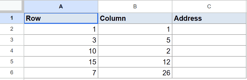
The goal is to convert each row and column pair into a standard cell reference in the Address column.

Here is the formula:

=ADDRESS(A2,B2)

Put it in C2 and fill it down through C6. Each row gets its own formula using the row and column values next to it.

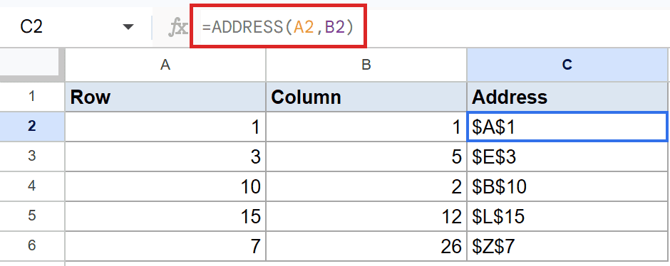
C2 returns $A$1, since row 1 and column 1 point at cell A1. The rest of the column fills in: $E$3 for row 3 column 5, $B$10 for row 10 column 2, $L$15 for row 15 column 12, and $Z$7 for row 7 column 26. By default ADDRESS returns the reference with both row and column locked using dollar signs.

Pro Tip: If you’d rather use a single formula instead of filling down, wrap ADDRESS in ARRAYFORMULA: =ARRAYFORMULA(ADDRESS(A2:A6,B2:B6)). The result spills into the same five cells. Per-row is easier to read for beginners, ARRAYFORMULA is cleaner once you’re comfortable with it.

Example 2: Switch between absolute, mixed, and relative styles

The third argument, absolute_relative_mode, controls whether the row and column come back locked with dollar signs or free to shift when the formula moves. There are four valid values: 1, 2, 3, and 4.

Below is a small table with the same row and column repeated four times, paired with each mode.

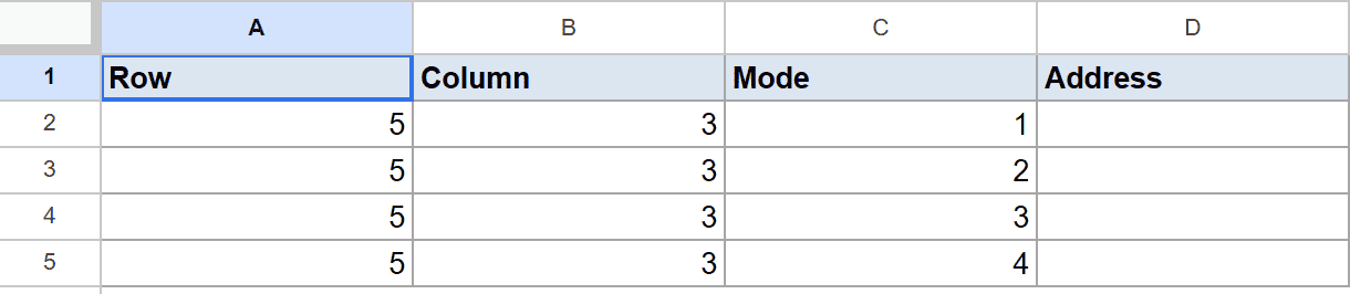
The goal is to see how the same row and column produce four different reference styles depending on the mode.

Here is the formula:

=ADDRESS(A2,B2,C2)

Put it in D2 and fill it down through D5.

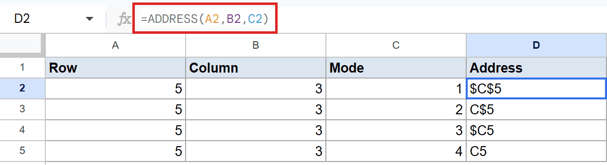
Each mode produces a different style for row 5, column 3:

• Mode 1 returns $C$5, with both row and column absolute. This is the default.
• Mode 2 returns C$5, with the row absolute and the column relative.
• Mode 3 returns $C5, with the column absolute and the row relative.
• Mode 4 returns C5, fully relative.

Picking the right mode matters when you plan to drop the resulting reference into another formula and then drag it. Locked references stay put, relative ones shift.

Pro Tip: To get R1C1 notation instead of A1, set the fourth argument to FALSE. =ADDRESS(5,3,1,FALSE) returns R5C3. Most users stick with A1, but R1C1 is sometimes handy when exporting to systems that expect that style.

Example 3: Include a sheet name in the returned address

The fifth argument lets you include a sheet name. ADDRESS will prepend that sheet name and the ! separator to the cell reference, giving you a fully-qualified cross-sheet address.

Below is a small table with row numbers, column numbers, and sheet names.

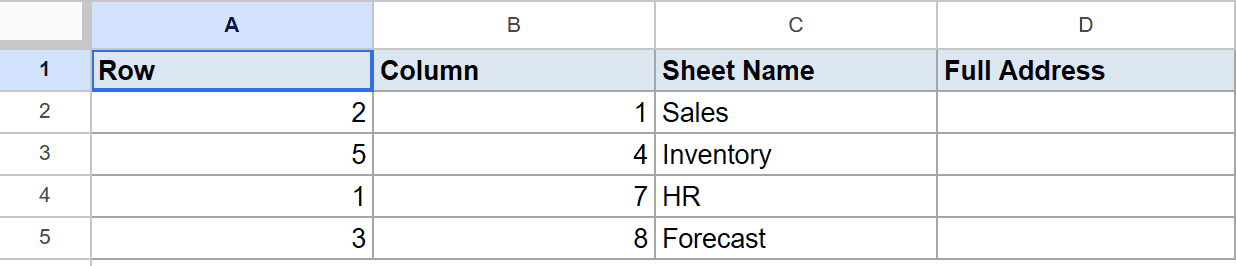
The goal is to build a full cross-sheet address for each row in the Full Address column.

Here is the formula:

=ADDRESS(A2,B2,1,TRUE,C2)

Put it in D2 and fill it down through D5. The middle arguments (mode 1, A1 notation) are passed explicitly because the sheet name has to be the fifth argument.

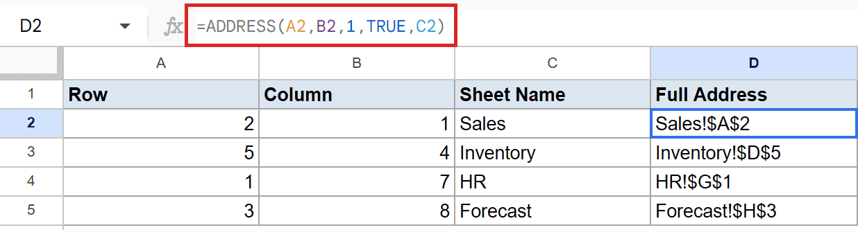
D2 returns Sales!$A$2. The other rows fill in similarly: Inventory!$D$5, HR!$G$1, and Forecast!$H$3. The text returned is ready to feed into a function like INDIRECT, as long as the sheet actually exists in the file.

Pro Tip: If your sheet name contains spaces or starts with a digit, Google Sheets expects single quotes around it in any real cell reference (for example 'Q1 Sales'!$A$1). ADDRESS does not add those quotes automatically, so you may need to wrap the sheet name yourself before passing the result to INDIRECT. A small tweak handles it: =ADDRESS(2,1,1,TRUE,"'Q1 Sales'").

Example 4: Fetch a value at a dynamic cell with ADDRESS and INDIRECT

ADDRESS by itself just returns text. To turn that text into a live cell reference and pull the value at that cell, wrap it in INDIRECT. This is where ADDRESS really earns its keep.

Below is a small lookup table with a row-to-fetch input and a column-to-fetch input.

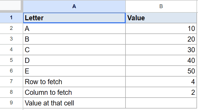
The goal is to pull the value at whatever cell the two inputs point to, without hard-coding the reference.

Here is the formula:

=INDIRECT(ADDRESS(B7,B8))

Put it in B9. B7 holds the row number (4) and B8 holds the column number (2).

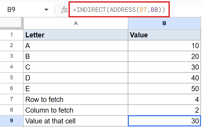
ADDRESS(B7, B8) builds the text $B$4. INDIRECT takes that text and turns it into a live reference to cell B4, which holds the value 30. Change the row or column input and the result updates instantly.

How this formula works:

• ADDRESS(B7, B8) reads the two input cells and returns the cell reference as text. With B7 = 4 and B8 = 2, this gives $B$4.
• INDIRECT(...) takes that text and treats it as a real reference, returning the value stored at that cell.
• Together, they let you point at a different cell just by changing the input numbers, with no formula edits needed.

Pro Tip: If both the data area and the inputs live on the same sheet, you don’t need the fifth argument. If the data is on another sheet, add the sheet name as the fifth argument to ADDRESS so INDIRECT knows where to look: =INDIRECT(ADDRESS(B7, B8, 1, TRUE, "Data")).

Example 5: Find the address of the largest value with ADDRESS and MATCH

ADDRESS pairs nicely with MATCH when you want to know which cell holds a particular value. MATCH returns the position of the value inside a range, and ADDRESS turns that position into a cell reference.

Below is a small table of salespeople and their sales totals.

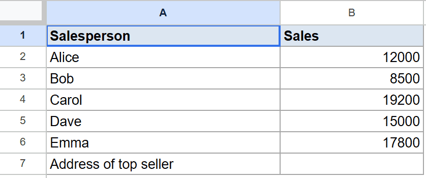
The goal is to find the cell address that holds the highest sales value.

Here is the formula:

=ADDRESS(MATCH(MAX(B2:B6),B2:B6,0)+1,2)

Put it in B7.

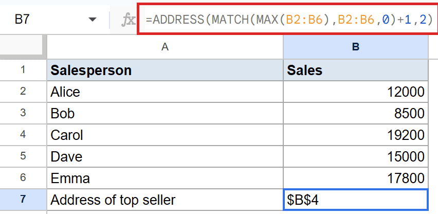
The formula returns $B$4, which is Carol’s sales cell. Carol has the top sales figure of 19,200, and her row in the sheet is row 4.

How this formula works:

• MAX(B2:B6) finds the largest value in the sales range, which is 19,200.
• MATCH(19200, B2:B6, 0) locates 19,200 at position 3 within B2:B6, since Carol’s row is the third entry in the range.
• Adding 1 to that position accounts for the header row, so the actual sheet row is 4.
• ADDRESS(4, 2) then returns $B$4, the cell that holds the maximum.

Pro Tip: If you want the salesperson’s name instead of the cell address, drop ADDRESS and use INDEX directly: =INDEX(A2:A6, MATCH(MAX(B2:B6), B2:B6, 0)) returns “Carol”. Use ADDRESS when you specifically need the cell reference itself, for example to feed into another formula or to display in an audit note.

Tips & Common Mistakes

• ADDRESS returns text, not a reference. A common mistake is expecting =ADDRESS(3,2) to fetch the value at B3. It won’t. It just returns the string $B$3. To get the value, wrap it in INDIRECT: =INDIRECT(ADDRESS(3,2)).
• Column number must match the column letter you expect. Column A is 1, not 0. So =ADDRESS(1,1) returns $A$1, and =ADDRESS(1,27) returns $AA$1. If you’re getting an unexpected column letter, double-check whether your formula is using a zero-based count somewhere upstream.
• Sheet names with spaces or special characters need quoting. ADDRESS will happily build Q1 Sales!$A$1 if you pass "Q1 Sales" as the sheet name, but that string is not a valid reference. Either avoid spaces in sheet names or wrap the name in single quotes when building the address: =ADDRESS(1,1,1,TRUE,"'Q1 Sales'") returns 'Q1 Sales'!$A$1, which is valid.

Closing thought. ADDRESS on its own is just a string builder, which is why it confuses people the first time they see it. The real value shows up the moment you pair it with INDIRECT or MATCH. Once that clicks, it becomes one of those small functions you reach for any time you need to point at a cell using numbers instead of typed-in references.

List of All Google Sheets Functions