FORMULATEXT Function in Google Sheets

If you want to see the actual formula sitting inside a cell, returned as plain text instead of its result, the FORMULATEXT function in Google Sheets does exactly that.

It is built for audit notes, documentation, training material, and any situation where the formula itself is the thing you need to display.

In this article, I’ll walk you through five practical examples that show how FORMULATEXT gets used in real spreadsheets, including how to pair it with IFERROR and string concatenation.

FORMULATEXT Function Syntax in Google Sheets

FORMULATEXT takes a single argument.

=FORMULATEXT(cell)

• cell: a reference to the cell whose formula you want returned as text. If the cell does not contain a formula, FORMULATEXT returns #N/A.

FORMULATEXT does not execute the formula. It only returns the formula as a string, exactly the way you typed it into the cell.

When to Use FORMULATEXT Function

• Show the formula behind a calculated cell without clicking into the cell.
• Document the formulas used in a calculation sheet for audits, reviews, or training.
• Label cells as either formula-driven or plain values, by pairing FORMULATEXT with IFERROR.
• Display a formula and its result side by side in a single cell using string concatenation.
• Build a screenshot-friendly view of a workbook where every formula is visible at a glance.

Example 1: See the formula behind a calculated cell

Let’s start with the simplest case. You have a column of calculated values, and you want to display the formula that produced each one in the next column.

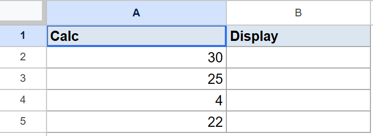
Below is a small table of calculations with their results in column B.

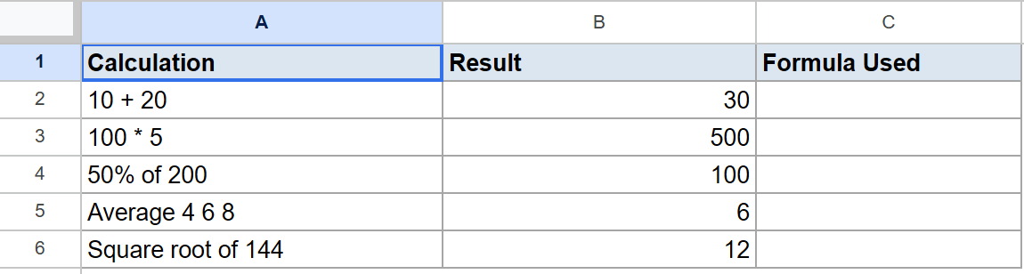
The goal is to show the underlying formula for each result in the Formula Used column.

Here is the formula:

=FORMULATEXT(B2)

Put it in C2 and fill it down through C6. Each row pulls the formula from the cell next to it.

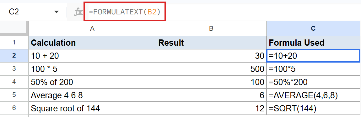
Each row in column C now shows the literal formula that produced the value in column B. =10+20 for the first row, =100*5 for the second, =50%*200, =AVERAGE(4,6,8), and =SQRT(144).

The point is that column B shows results, while column C shows the formula text exactly as you typed it, even though both columns point at the same cells.

Pro Tip: FORMULATEXT returns the formula as text, which means leading = signs come along with it. If you want only the body of the formula without the equals sign, wrap it in MID: =MID(FORMULATEXT(B2),2,LEN(FORMULATEXT(B2))). Useful for cleaner audit reports.

Example 2: Document formulas in a calculation sheet for audit

When someone hands off a workbook, the fastest way to make it auditable is to show each metric next to the formula that produced it. FORMULATEXT makes that a one-liner.

Below is a small calculation sheet with four metrics and their formula-driven values in column B.

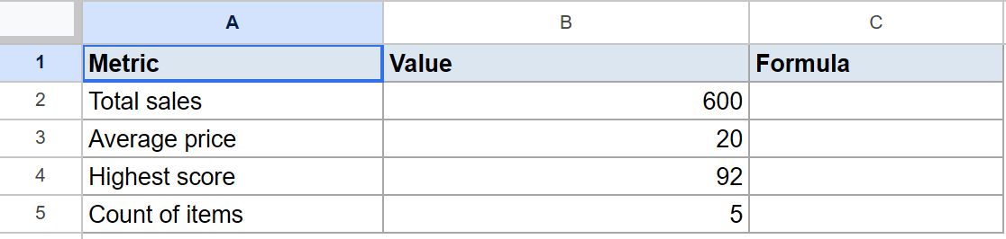
The goal is to fill column C with the formula text that produced each value in column B.

Here is the formula:

=FORMULATEXT(B2)

Put it in C2 and fill it down through C5.

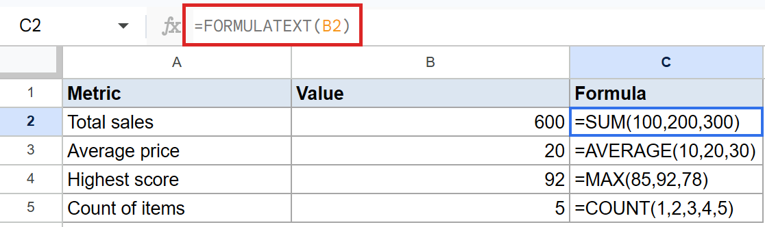
Column C now reads =SUM(100,200,300), =AVERAGE(10,20,30), =MAX(85,92,78), and =COUNT(1,2,3,4,5). A reviewer can see the metric, the result, and the formula in one pass, without clicking into every cell. If anyone edits a formula in column B, column C updates instantly.

That live link is what makes FORMULATEXT useful for documentation, not just static screenshots.

Pro Tip: To freeze the formula text so it doesn’t change when the source formula gets edited, copy the FORMULATEXT column and paste it as values. Now you have a permanent record of what the formulas were at the time of the audit.

Example 3: Label cells as formula or plain value with IFERROR

FORMULATEXT returns #N/A when the target cell contains a plain value, a blank, or text.

That error is not a bug, it is the signal you need to label cells as formula-driven or not. Wrap it in IFERROR and you have a clean yes-or-no check.

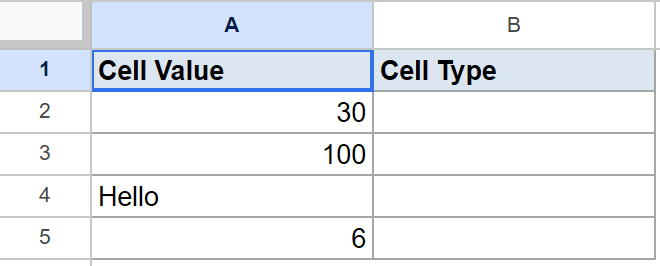
Below is a small list of cell contents in column A. Some are formulas, some are plain values, and some are text.

The goal is to tag each cell in column B as either a formula (showing the formula text) or a plain value.

Here is the formula:

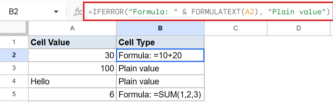
=IFERROR("Formula: " & FORMULATEXT(A2), "Plain value")

Put it in B2 and fill it down through B5.

How this formula works:

• FORMULATEXT(A2) tries to fetch the formula in A2. If A2 holds a formula, it returns the formula text. If A2 holds a plain value or text, it returns #N/A.
• "Formula: " & FORMULATEXT(A2) prepends the label Formula: to the formula text, but only when FORMULATEXT succeeds.
• IFERROR(..., "Plain value") catches the #N/A from plain-value cells and returns the fallback string Plain value instead.

The result is Formula: =10+20 for the first cell, Plain value for 100, Plain value for “Hello”, and Formula: =SUM(1,2,3) for the last cell.

Pro Tip: If you only need a TRUE-or-FALSE flag instead of a label, use ISFORMULA: =ISFORMULA(A2) returns TRUE for formula cells and FALSE for everything else. FORMULATEXT and ISFORMULA cover the same ground but ISFORMULA is cleaner when you only need a yes-or-no.

Example 4: Show the formula used in a totals row

Totals rows often carry the most important formula on the sheet, but they sit at the bottom where reviewers may not click.

Surfacing the formula text right below the totals row makes the calculation visible without any extra effort.

Below is a small quantities table with a totals row at the bottom.

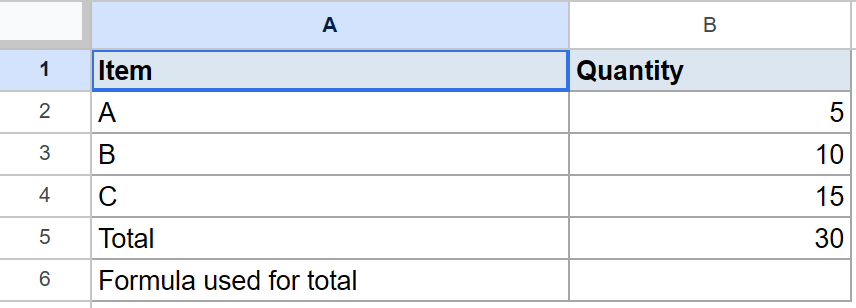
The goal is to show the SUM formula driving the total directly underneath it.

Here is the formula:

=FORMULATEXT(B5)

Put it in B7.

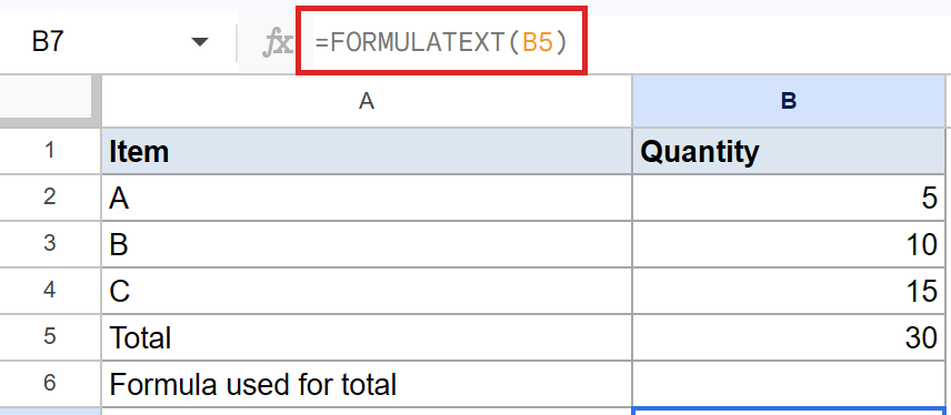
B7 returns =SUM(B2:B4). If you change the totals formula to =SUMPRODUCT(B2:B4,1) or add a new row and update the range, B7 updates to reflect the new formula.

Useful for templates that get handed around the team, where the totals formula sometimes drifts and you want a visible record of what’s actually doing the math.

Pro Tip: Pair FORMULATEXT with conditional formatting to highlight rows where the formula deviates from a standard pattern. For example, flag any total cell whose formula does not start with =SUM. That helps catch one-off edits during reviews.

Example 5: Display formula and its result together in one cell

A self-documenting cell shows both the formula and what it evaluates to.

Useful for printed worksheets, classroom handouts, and quick visual references where you want the reader to see the math and the answer side by side.

Below is a small list of formulas in column A. Each one is a real formula that returns a number.

The goal is to build a display string in column B that shows both the formula and its computed result.

Here is the formula:

=FORMULATEXT(A2) & " = " & A2

Put it in B2 and fill it down through B5.

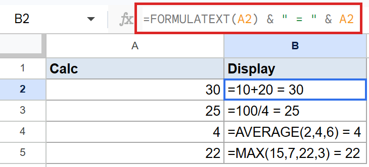
How this formula works:

• FORMULATEXT(A2) returns the formula text from A2, for example =10+20.
• " = " is a literal connector string that sits between the formula and the result.
• A2 returns the computed result of the formula, for example 30.
• The & operator joins the three pieces into one string: =10+20 = 30.

The other rows produce =100/4 = 25, =AVERAGE(2,4,6) = 4, and =MAX(15,7,22,3) = 22. Each cell is now self-documenting, showing both the formula and the answer in one line.

Pro Tip: If your cell values are dates, percentages, or currency, use TEXT to format the result side: =FORMULATEXT(A2) & " = " & TEXT(A2, "0.00%"). That keeps the display consistent with the way the source cells are formatted.

Tips & Common Mistakes

• FORMULATEXT returns #N/A on plain values. That is not a bug, it is the function telling you the cell does not have a formula. If you want a clean label instead, wrap FORMULATEXT in IFERROR or use ISFORMULA for a TRUE-or-FALSE check.
• Empty cells also return #N/A. A blank target cell is not a formula, so FORMULATEXT treats it the same way as a plain value. The IFERROR wrapper handles this case too.
• The text updates live as the source formula changes. FORMULATEXT is not a snapshot. If you edit the formula in B2, every FORMULATEXT pointing at B2 refreshes instantly. To freeze the formula text, copy the FORMULATEXT cells and paste them as values.

FORMULATEXT is a small function with a narrow job, but it shows up in any workflow where the formula itself is the deliverable.

Audit reviews, training material, printed worksheets, and template handoffs all benefit from having the formula text visible alongside the result.

Pair it with IFERROR or ISFORMULA and you have a complete toolkit for inspecting what’s living inside your cells.

List of All Google Sheets Functions