If you want to embed a picture inside a cell from a URL, the IMAGE function in Google Sheets does it in one step. Pass it the web address of an image and the picture loads right inside the cell.
In this article, I’ll show you how to use IMAGE with the default mode, the three explicit sizing modes, and the custom pixel-size mode for grid-aligned thumbnails.
IMAGE Function Syntax in Google Sheets
The IMAGE function embeds an image inside a cell from a URL.
=IMAGE(url, [mode], [height], [width])
- url is the public web address of the image, in quotes or as a cell reference. The link must be reachable without sign-in.
- mode is optional. 1 fits the image inside the cell and keeps the aspect ratio (this is the default). 2 stretches the image to fill the cell and ignores the aspect ratio. 3 keeps the image at its native pixel size. 4 takes a custom pixel height and width.
- height and width are pixel sizes for mode 4 only. Height comes first, then width.
The cell holds a rendered picture, not a value. You usually need to widen the row before you can actually see the image.
When to Use IMAGE Function
- Embed product photos next to product names in an inventory sheet.
- Add a small logo to a dashboard cell without a separate image object.
- Show profile pictures next to employee or customer rows.
- Pair it with a lookup function to swap an image based on a selection.
- Build a quick visual price list or catalog directly in the sheet.
Example 1: Embed an Image With the Default Mode
Let’s start with the simplest call, passing just the URL.
Below is the dataset. Column A has three picsum.photos URLs, one for a black dog, one for a mountain landscape, and one for a forest scene. Column B is where the rendered images will land.
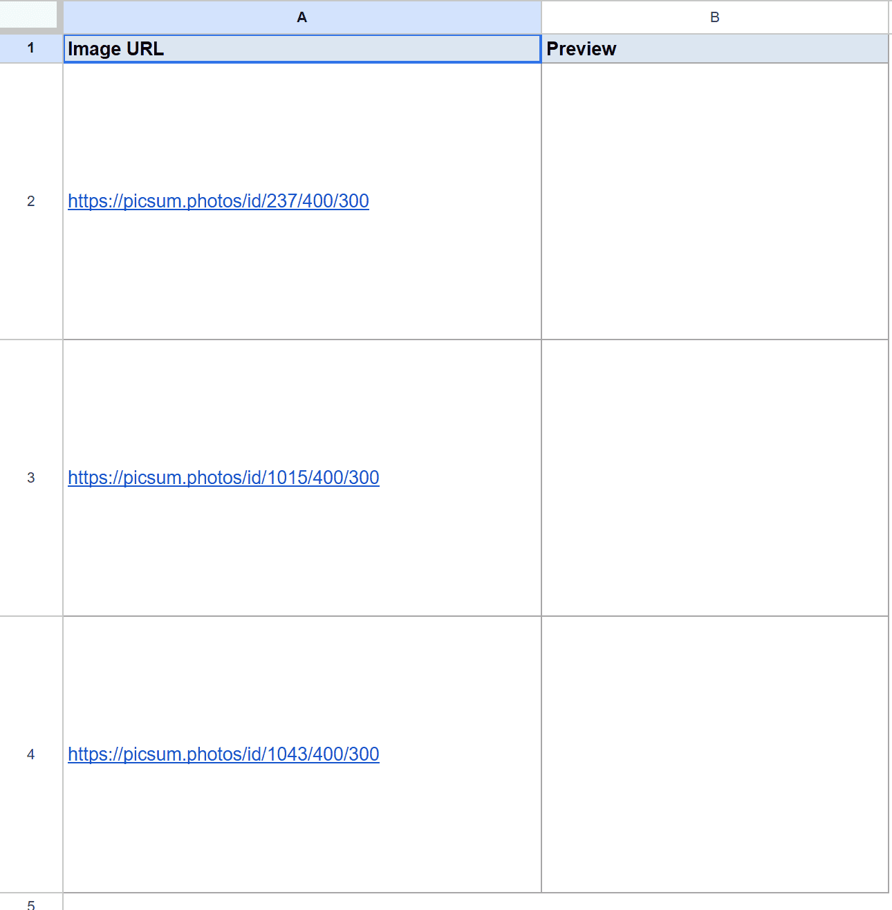
I want each picture to load into the matching row of column B.
Here is the formula:
=IMAGE(A2)
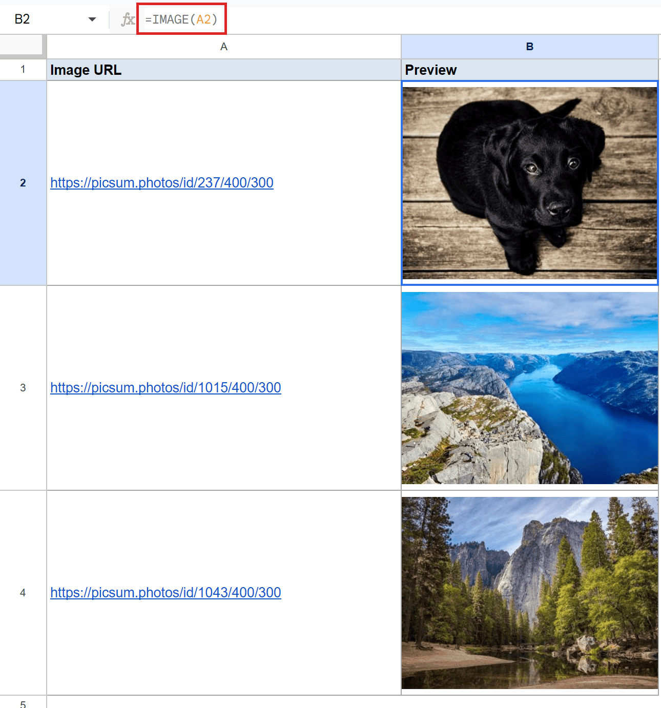
The default mode fits the picture inside the cell and keeps its original aspect ratio. Each row in column B now shows the photo at column A’s URL, scaled to fit the cell width with the height adjusted to match.
If the row is still its default 21 pixels tall, the image will look like a tiny strip. Drag the row border down until you can see the full picture.
Pro Tip: To resize multiple rows at once, click the row 2 header, shift-click the last row header, then right-click and pick Resize rows. Set a fixed height like 80 or 100 pixels and every selected row updates in one go.
Example 2: Fit to Cell Explicitly With Mode 1
The same three URLs again, this time passing mode 1 explicitly.
Below is the dataset. Same three picsum.photos URLs as Example 1, in column A.

I want to confirm that mode 1 behaves the same as the default.
Here is the formula:
=IMAGE(A2, 1)
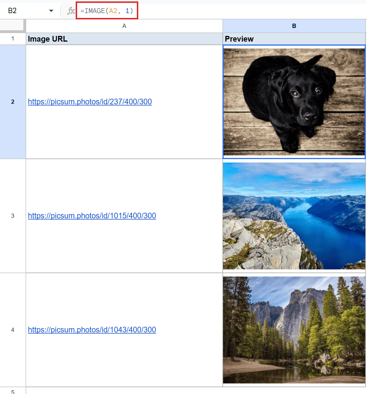
Mode 1 is identical to the default mode. The picture fits inside the cell and keeps its original aspect ratio. Each image in column B looks the same as it did in Example 1.
Use mode 1 when you want to be explicit about the sizing behavior, for example when other examples in the same sheet use a different mode and you want all the formulas to read consistently.
Example 3: Stretch to Fill the Cell With Mode 2
Mode 2 changes how the picture fits the cell.
Below is the dataset. Same three picsum.photos URLs as before, so the only change from Example 1 is the mode argument.

I want each picture to fill the entire cell, even if that means distorting it.
Here is the formula:
=IMAGE(A2, 2)
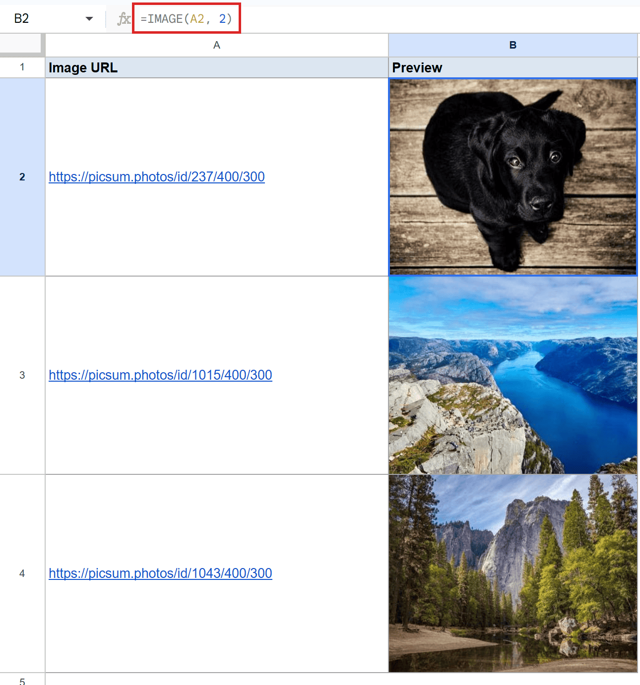
Mode 2 stretches the picture to fill the cell in both directions and ignores the aspect ratio. The original photos are wider than they are tall (400 by 300 pixels), so in a narrower cell they end up squished horizontally. In a taller cell they end up stretched vertically.
This mode is rarely what you want for product photos or portraits since people look distorted. It is fine for textures, backgrounds, or any image where shape doesn’t matter.
Example 4: Keep the Original Image Size With Mode 3
Mode 3 ignores the cell size entirely.
Below is the dataset. Same three URLs as Example 1 in column A.

I want each picture to render at its native pixel size, regardless of how big the cell is.
Here is the formula:
=IMAGE(A2, 3)
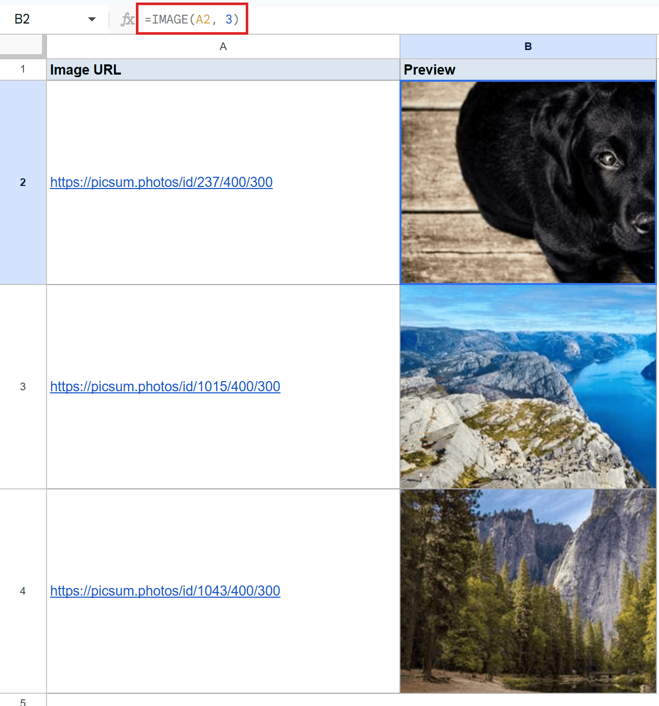
Mode 3 renders the image at its native pixel size. The picsum.photos URLs all serve 400 by 300 pixel images, so each picture tries to take up 400 by 300 pixels of cell space.
If the cell is smaller than the image, the picture overflows or gets clipped. If the cell is bigger, the picture sits in the top-left with empty space around it. To use mode 3 well, resize the column and row to match the image dimensions first.
Example 5: Set a Custom Height and Width With Mode 4
Mode 4 lets you pick an exact size.
Below is the dataset. Same three picsum.photos URLs.

I want every picture to render at the same fixed dimensions, 80 pixels tall by 120 pixels wide.
Here is the formula:
=IMAGE(A2, 4, 80, 120)
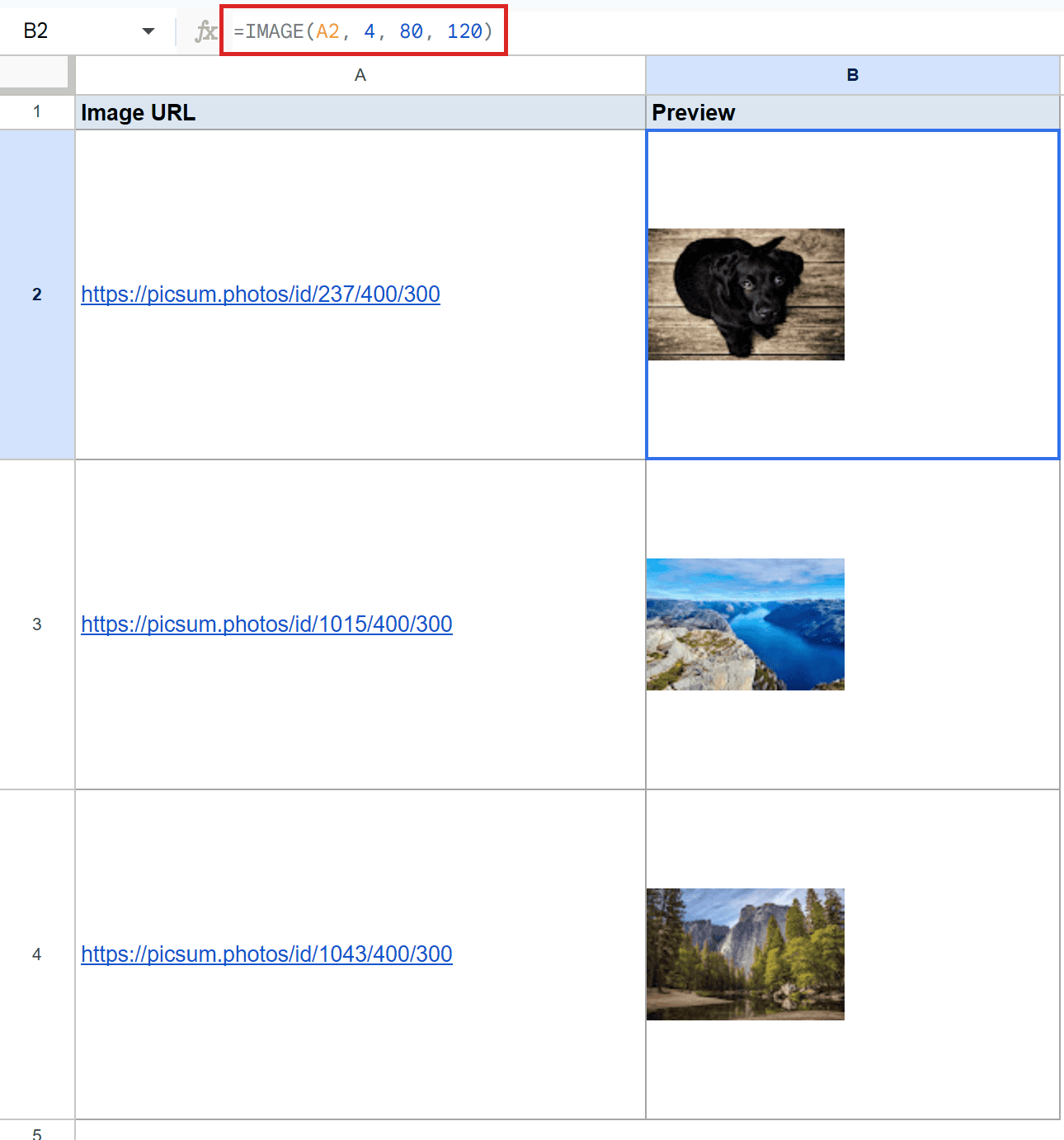
Mode 4 takes the pixel height and width as the third and fourth arguments. Notice the order, height first then width. That’s the opposite of how most image specs read.
Every picture now sits at exactly 80 by 120 pixels, perfect for a uniform grid of thumbnails. Resize the row to at least 80 pixels and the column to at least 120 pixels so the images aren’t clipped.
Pro Tip: Combine IMAGE with a lookup function like HLOOKUP or LOOKUP to swap the picture based on a dropdown selection. Store the URLs in a hidden lookup table, point the lookup at the user’s choice, and wrap the result in IMAGE. The cell becomes a live photo that updates when the dropdown changes.
Tips & Common Mistakes
- Resize the row to see the picture. IMAGE renders the picture inside the cell, but if the row is at the default 21 pixel height the image gets squished into a sliver. Drag the row border down, or right-click the row header and pick Resize rows, until you can actually see the photo.
- The URL must be public. IMAGE needs to fetch the file without sign-in. A Google Drive link only works if the file is shared with “Anyone with the link”. A link behind a login or hotlink-protection breaks the formula with #VALUE! or #N/A. Test the URL in an incognito browser tab first.
- Mode 4 takes height before width. It’s the opposite order from most image specs you’ve seen. =IMAGE(url, 4, 80, 120) makes an 80-pixel-tall, 120-pixel-wide picture. Swap them and you’ll get a tall narrow image instead of a short wide one.
- Max 2 MB per image, 1500 by 1500 pixels. Beyond that limit the cell breaks with an error. Resize or compress the source image first, or host a smaller version on a public cloud bucket with anonymous read access.
IMAGE pulls a public picture into a cell from a URL. The default mode fits the image inside the cell while keeping its shape, and three more modes let you stretch, keep the native size, or pick exact pixel dimensions.
The real-world use cases are product galleries, dashboard logos, employee or customer photos, and lookup-driven catalogs where the picture changes based on a dropdown. Once you’ve widened the row and confirmed the URL is public, IMAGE handles the rest.