
TIME in Google Sheets builds a time of day from separate hour, minute, and second values. For example, =TIME(14,30,0) represents 2:30 PM. Format the result as Time to display a clock value.
Build a Time from Three Columns
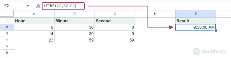
Enter this dataset starting in A1. Leave cells marked “(blank)” empty.
| Hour | Minute | Second |
|---|---|---|
| 9 | 30 | 0 |
| 14 | 30 | 0 |
| 23 | 59 | 59 |
Enter this formula in E2:
=TIME(A2,B2,C2)The result is 9:30:00 AM. In the menu, choose Format → Number → Time if the result appears as a decimal. The underlying value is approximately 0.3958333333.
TIME Function Syntax
=TIME(hour, minute, second)All three arguments are required. Use numeric components, with 0 for any unused minutes or seconds. Typical clock inputs are hours 0–23 and minutes and seconds 0–59.
TIME stores a fraction of a day: noon is 0.5 and midnight is 0. The function represents a time of day; it is not a reliable container for a duration exceeding 24 hours.
To process all three example rows with one formula, enter this in an empty column:
=ARRAYFORMULA(TIME(A2:A4,B2:B4,C2:C4))The outputs are 9:30:00 AM, 2:30:00 PM, and 11:59:59 PM. Apply Time formatting to the output range, and leave its three cells clear for expansion.
Understand Overflow and Decimal Components
=TIME(25,30,0)The result is 1:30 AM. TIME wraps hours beyond 23. Similarly, =TIME(9,90,0) returns 10:30 AM because 90 minutes adds an hour and 30 minutes.
Decimal components are truncated individually. =TIME(9.9,30.9,0.9) returns 9:30 AM, not 9.9 hours plus 30.9 minutes. Validate inputs first if overflow or fractional components should be rejected.
Create a Fixed Afternoon Time
=TIME(14,30,0)This returns 2:30 PM after Time formatting. Its stored value is approximately 0.6041666667. Numeric components avoid relying on recognition of a typed text string such as “2:30 PM”.
Add or Subtract Minutes
=TIME(9,0,0)+TIME(0,30,0)The result is 9:30 AM. Replace the first TIME expression with a cell containing your start time. To subtract 15 minutes from 9:00 AM, use:
=TIME(9,0,0)-TIME(0,15,0)That returns 8:45 AM. Minutes are represented as fractions of a day, which is why these values can be added and subtracted numerically.
Calculate a Shift End and Handle Midnight
Enter this dataset starting in A12. Leave cells marked “(blank)” empty.
| Start | Hours | Minutes |
|---|---|---|
| =TIME(8,0,0) | 8 | 0 |
| =TIME(9,30,0) | 7 | 30 |
| =TIME(23,30,0) | 2 | 0 |
=A13+TIME(B13,C13,0)The first shift ends at 4:00 PM. Filling down gives 5:00 PM and 1:30 AM. The last result includes a whole day internally because the addition crosses midnight.
That day is retained by addition, although Time formatting hides it. This differs from passing 25 hours directly into TIME, which discards the whole day while constructing the time.
For 25.5 elapsed hours, use =25.5/24 and choose Format → Number → Duration. This preserves the complete duration rather than wrapping to 1:30 AM.
Combine a Date and a Time
=DATE(2026,1,15)+TIME(9,30,0)Format the result as Date time to display January 15, 2026 at 9:30 AM. Combining a date with the clock time keeps the calendar day available for later calculations.
Other Google Sheets articles you may also like
- Build a date from numeric components
- Get the current date and time