
If you want to pull only the rows that meet a condition out of a larger range, the FILTER function in Google Sheets does it in a single formula.
You hand it a range and one or more tests, and it returns just the matching rows. The results spill into the cells below. In this article I’ll show you how it works with five examples, including how to test on two conditions at once.
FILTER Function Syntax in Google Sheets
Here is how you write the FILTER function.
=FILTER(range, condition1, [condition2, ...])
- range – the data you want to filter. This is what gets returned, minus the rows that fail.
- condition1 – a test that lines up row-for-row with the range. Rows where it’s TRUE are kept.
- condition2, … – optional extra tests. By default they all have to pass for a row to stay.
When to Use FILTER Function
- Show only rows that beat a threshold, like scores at or above 85.
- Pull every row for one category, like a single department or region.
- Apply two tests at once, keeping rows that pass both.
- Match either of two values using an OR condition.
- Return one column from a table based on a test in another column.
Example 1: Filter Rows Above a Threshold
Let’s start with a single numeric test.
Below is the dataset, a list of names in column A and their scores in column B.
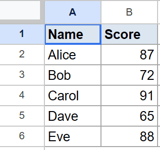
The goal is to return only the people who scored 85 or higher.
Here is the formula:
=FILTER(A2:B6, B2:B6>=85)
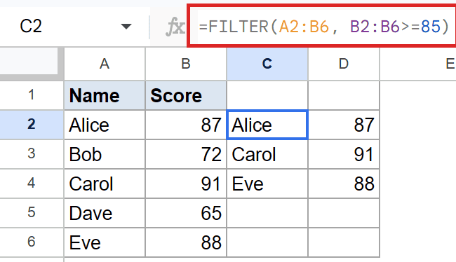
The condition B2:B6>=85 checks each score and marks the row TRUE or FALSE. FILTER keeps the TRUE rows and drops the rest.
You get three rows back, Alice at 87, Carol at 91, and Eve at 88. Notice there’s no header row in the output. FILTER returns only the matching data.
Pro Tip: The condition range has to be the same height as the range you’re filtering. Filtering A2:B6 means your test also has to span five rows, like B2:B6. A mismatch throws an error.
Example 2: Filter by a Text Match
Now let’s filter on a text value instead of a number.
Below is the dataset, with employee names in column A, their department in column B, and salary in column C.
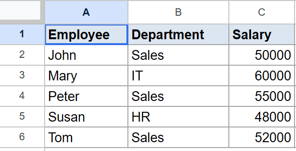
The goal is to return everyone in the Sales department, with all their columns.
Here is the formula:
=FILTER(A2:C6, B2:B6="Sales")
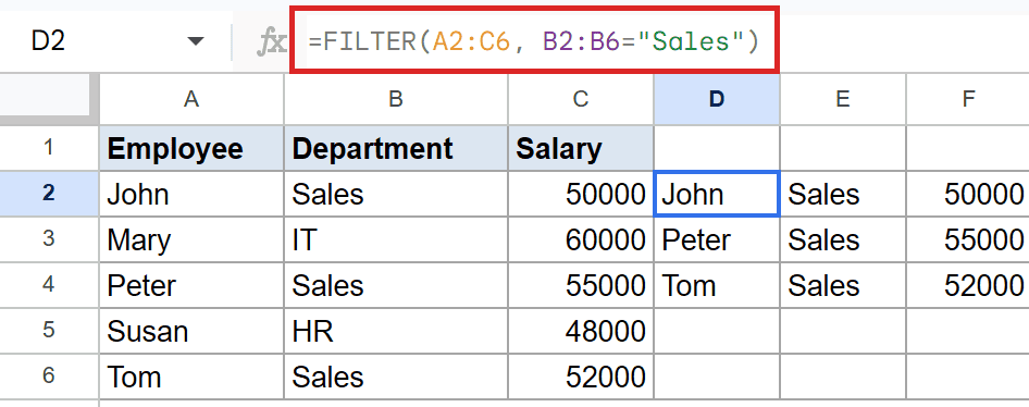
The condition B2:B6="Sales" is TRUE for every row where the department reads Sales. Text comparisons go in double quotes inside the formula.
Three rows come back, John, Peter, and Tom, each with their department and salary intact. The whole row carries through, not just the name.
Example 3: Apply Two Conditions
Here you can stack two tests, and a row has to clear both.
Below is the dataset, a fruit list in column A, units in column B, and price in column C.
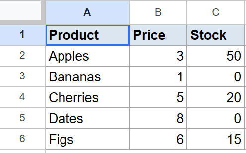
The goal is to keep rows where the price is positive and the units are above 4.
Here is the formula:
=FILTER(A2:C6, C2:C6>0, B2:B6>4)
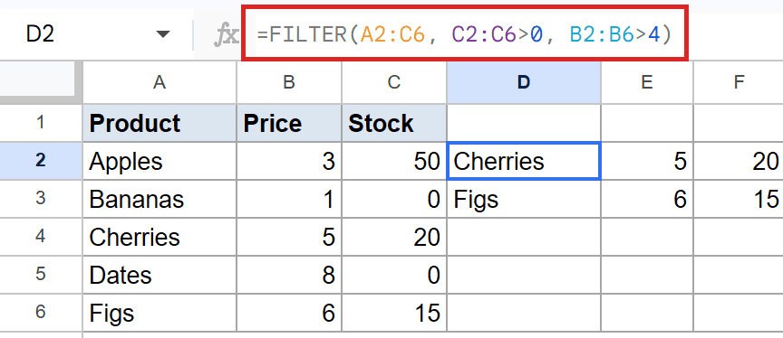
When you list more than one condition, FILTER treats them as AND. A row survives only if every test is TRUE.
How this formula works:
C2:C6>0keeps rows with a price above zero.B2:B6>4keeps rows with more than 4 units.
Only Cherries and Figs pass both checks. Cherries shows 5 units at a price of 20, and Figs shows 6 units at a price of 15.
Example 4: Match Either of Two Values
What if you want rows matching one value OR another? You add the conditions together.
Below is the dataset, a city in column A and an amount in column B.
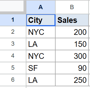
The goal is to keep every row where the city is NYC or LA.
Here is the formula:
=FILTER(A2:B6, (A2:A6="NYC")+(A2:A6="LA"))
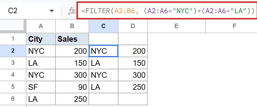
Adding two conditions with + is how you do OR in FILTER. A row passes if either test is TRUE, since the sum then comes out greater than zero.
Four rows come back, NYC with 200, LA with 150, NYC with 300, and LA with 250. Only rows for other cities get filtered out.
Pro Tip: Use + for OR and * for AND when you combine conditions inside one set of parentheses. Listing conditions as separate arguments is always AND, so + is the way to express OR.
Example 5: Return One Column Based on Another
You don’t have to return the whole range. You can pull a single column.
Below is the dataset, an order ID in column A, a customer name in column B, and an amount in column C.
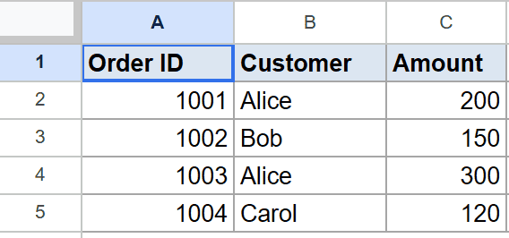
The goal is to return only the order IDs that belong to Alice.
Here is the formula:
=FILTER(A2:A5, B2:B5="Alice")
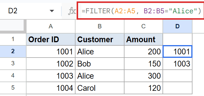
The range here is just column A, the order IDs. The condition tests column B, the customer name, for Alice.
Two order IDs come back, 1001 and 1003. The range you return and the column you test on can be different, as long as they line up row-for-row.
Tips & Common Mistakes
- The condition has to be the same height as the range you’re filtering. Filtering five rows means the test must cover five rows too, or you’ll get an error.
- For OR logic, add conditions with +. For AND, either list them as separate arguments or multiply them with *.
- FILTER returns no header row. If you want a header above the results, type it in the cell above the formula yourself.
FILTER is the function to reach for whenever you want a clean subset of your data without sorting, copying, or deleting anything. The source stays untouched, and the result updates the moment your data changes.
Start with one condition, then add a second or switch to + for OR as your needs grow. The five examples above cover most everyday filtering jobs.
List of All Google Sheets Functions
Related Google Sheets Functions / Articles: