
The SUMIFS function in Google Sheets adds numbers only when every condition you provide is met. It is ideal for totals by region, product, date, owner, or value range.
The tested examples below move from two conditions to criteria cells, date boundaries, wildcards, nonblank cells, and OR logic.
SUMIFS Function Syntax in Google Sheets
=SUMIFS(sum_range, criteria_range1, criterion1, [criteria_range2, criterion2, ...])
- sum_range contains the numbers to add.
- criteria_range1 contains the values tested by the first rule.
- criterion1 is the first value, reference, expression, or pattern to match.
- Additional range and criterion pairs add more required conditions.
Every criteria range must match the size of the sum range. SUMIFS uses AND logic, so a row contributes only when all criteria are true.
Unlike SUMIF in Google Sheets, SUMIFS puts the sum range first. SUMIF places its optional sum range last.
Sum with Two or Three Conditions
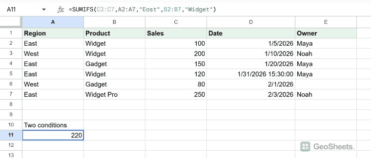
The fixture uses Region in column A, Product in B, Sales in C, Date in D, and Owner in E.
| Region | Product | Sales | Date | Owner |
|---|---|---|---|---|
| East | Widget | 100 | Jan 5, 2026 | Maya |
| West | Widget | 200 | Jan 10, 2026 | Noah |
| East | Gadget | 150 | Jan 20, 2026 | Maya |
| East | Widget | 120 | Jan 31, 2026, 3:30 PM | Maya |
| West | Gadget | 80 | Feb 1, 2026 | |
| East | Widget Pro | 250 | Feb 3, 2026 | Noah |
Total East Widget sales
=SUMIFS(C2:C7,A2:A7,"East",B2:B7,"Widget")
Two East rows contain the exact product Widget, with sales of 100 and 120. SUMIFS returns 220.
SUMIFS evaluates each row against East and Widget. Only rows passing both tests contribute their Sales value from column C.
Add an owner condition
=SUMIFS(C2:C7,A2:A7,"East",B2:B7,"Widget",E2:E7,"Maya")
The same two rows also belong to Maya, so the result remains 220. Any row failing one of the three tests is excluded.
Adding another criteria pair narrows the total. Criteria order does not change the arithmetic when each range still aligns with the same rows.
Use Cell References as SUMIFS Criteria
Enter East in H2 and Widget in H3. Then use:
=SUMIFS(C2:C7,A2:A7,H2,B2:B7,H3)
The formula returns 220. Changing either input cell recalculates the total without changing the formula itself.
Criteria cells work well for small summary panels. Labels and input cells can sit beside the source table while the formula remains stable.
Sum Numbers Inside a Range
=SUMIFS(C2:C7,C2:C7,">=100",C2:C7,"<=200")
Both criteria inspect the Sales column. Values from 100 through 200 are included, producing a total of 570.
Using the same column for the sum range and both criteria ranges creates a bounded total. The lower and upper comparisons are both inclusive.
Comparison operators belong inside quotation marks. When the boundary comes from a cell, join the operator and reference, such as ">="&H2.
Sum a Date Range Without Missing Timestamps
Use an inclusive start and an exclusive first day of the next month:
=SUMIFS(C2:C7,D2:D7,">="&DATE(2026,1,1),D2:D7,"<"&DATE(2026,2,1))
This formula returns 570 for January. It includes the 120 sale recorded on January 31 at 3:30 PM.
DATE also avoids ambiguous typed date text. The sheet interprets its year, month, and day arguments consistently with the formula.
This month-boundary pattern works for any month. Change both DATE expressions so the second date is the first day after the reporting period.
Match Partial Text with Wildcards
=SUMIFS(C2:C7,A2:A7,"East",B2:B7,"Widget*")
The asterisk matches any sequence after Widget. The result is 470 because the formula includes East rows for Widget and Widget Pro.
Sum Rows with Nonblank Criteria Cells
=SUMIFS(C2:C7,A2:A7,"East",E2:E7,"<>")
The <> criterion means not blank. Every East row in the fixture has an owner, so the result is 620.
Apply the nonblank test to the field that makes a record complete, such as Owner, invoice number, or approval date.
Use OR Logic in SUMIFS
SUMIFS requires all criteria in one call. For mutually exclusive alternatives, add separate SUMIFS results:
=SUMIFS(C2:C7,A2:A7,"East",B2:B7,"Widget")+SUMIFS(C2:C7,A2:A7,"West",B2:B7,"Widget")
The first part returns 220 and the second returns 200, giving 420. A row cannot be both East and West, so nothing is counted twice.
To count matching rows instead of adding their values, use the COUNTIFS function.
Fix SUMIFS Range and No-Match Results
A no-match result is zero
=SUMIFS(C2:C7,A2:A7,"North")
The fixture has no North rows, so SUMIFS returns 0. This differs from FILTER, which returns #N/A when nothing matches.
Mismatched range sizes return an error
=SUMIFS(C2:C7,A2:A6,"East") returns #VALUE!. The six-cell sum range does not align with the five-cell criteria range.
Check the first and last row of every range when this error appears. Whole-column references should also use matching whole columns.
Other Google Sheets articles you may also like