
If you want to strip the duplicates out of a list and keep just one of each value, the UNIQUE function in Google Sheets does it in one step. It reads your range and spills back only the distinct entries.
In this article, I’ll show you how UNIQUE works, walk through four practical examples, and point out a couple of things to keep in mind.
UNIQUE Function Syntax in Google Sheets
The UNIQUE function takes a range and returns its distinct rows.
=UNIQUE(range, [by_column], [exactly_once])
- range is the data you want the distinct values from.
- by_column is optional. Set it TRUE to compare columns instead of rows. Defaults to FALSE.
- exactly_once is optional. Set it TRUE to keep only values that appear a single time. Defaults to FALSE.
The result spills into the cells below the formula, so leave room for it.
When to Use UNIQUE Function
Here are a few times UNIQUE comes in handy.
- Building a clean list of distinct regions, products, or names from messy data.
- Pulling the unique combinations across two or more columns.
- Feeding a deduplicated list into another function like SORT or COUNTA.
- Setting up a dropdown source that has no repeats.
Example 1: Unique Values from a Single Column
Let’s start with the most common use.
Below is the dataset, a single column of regions with several repeats in it.
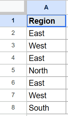
The goal is to get a list of each region just once.
Here is the formula:
=UNIQUE(A2:A8)
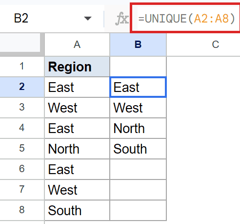
UNIQUE reads the column, drops the repeated regions, and spills the distinct ones down the cells below. The seven entries collapse into four unique regions, in the order they first appear.
Pro Tip: UNIQUE keeps the first-seen order of your data. If you want the list alphabetized instead, wrap it in SORT, which you’ll see in Example 3.
Example 2: Unique Rows from a Two Column Range
UNIQUE works across multiple columns, not just one.
Below is the dataset, with a fruit in column A and a color in column B, where some full rows repeat.
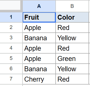
The goal is to find the distinct fruit-and-color combinations.
Here is the formula:
=UNIQUE(A2:B7)
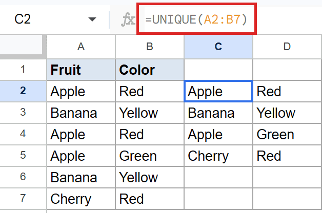
UNIQUE compares whole rows here, not single cells. Apple-Red shows up twice but counts once, while Apple-Green is kept because the color differs. Six rows become four distinct combinations.
Pro Tip: When you pass more than one column, UNIQUE treats each entire row as the thing to dedupe. Two rows have to match in every column to be counted as a duplicate.
Example 3: Unique Names Sorted Alphabetically with SORT
You can clean up the order by wrapping UNIQUE in SORT.
Below is the dataset, a single column of names with a few repeats.
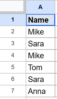
The goal is to get the distinct names in alphabetical order.
Here is the formula:
=SORT(UNIQUE(A2:A7))
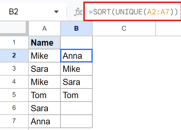
How this formula works:
- UNIQUE first reduces the list to the distinct names.
- SORT then arranges those names alphabetically.
- The four unique names come back in A-to-Z order instead of first-seen order.
Example 4: Counting Distinct Entries with COUNTA and UNIQUE
You can count how many distinct values there are by combining two functions.
Below is the dataset, a single column of quarter labels with plenty of repeats.
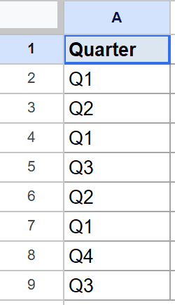
The goal is to count how many different quarters appear, not how many rows there are.
Here is the formula:
=COUNTA(UNIQUE(A2:A9))
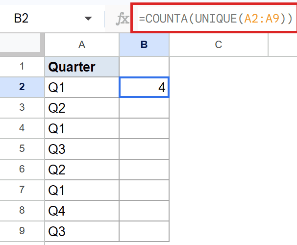
How this formula works:
- UNIQUE narrows the eight rows down to the distinct quarters.
- COUNTA then counts how many values came back from UNIQUE.
- The count of distinct quarters is 4.
Pro Tip: If counting distinct values is all you need, the COUNTUNIQUE function does it directly in one call, no UNIQUE wrapper required.
Tips & Common Mistakes
- Leave room for the spill. UNIQUE writes its results into the cells below the formula. If something is already sitting there, you’ll get a
#REF!error until you clear that space. - It’s case sensitive. UNIQUE treats “Open” and “open” as two different values, so normalize the case first if you don’t want them split apart.
- Blank rows can sneak in. An empty cell inside your range can show up as a blank entry in the result. Trim your range to the data, or filter the blanks out first.
UNIQUE pulls the distinct values out of a range and spills them into the cells below, dropping every duplicate along the way. You saw it dedupe a single column, handle two columns at once, pair with SORT for an ordered list, and team up with COUNTA for a distinct count.
Keep the spill space and case sensitivity in mind and it’s a fast way to clean up repeated data.
List of All Google Sheets Functions
Related Google Sheets Functions / Articles: