FLATTEN Function in Google Sheets

Sometimes you have data spread across rows and columns but need it stacked into a single tall list. The FLATTEN function in Google Sheets does exactly that in one call.

This article walks through four FLATTEN examples, from collapsing a 2D grid to combining columns and pulling unique items.

FLATTEN Function Syntax in Google Sheets

FLATTEN takes one or more ranges and stacks every value into a single column, reading left-to-right and top-to-bottom.

=FLATTEN(range1, [range2, ...])
  • range1 – the first range to flatten into a column
  • range2, … – additional ranges to append below the first one, [optional]

When to Use FLATTEN Function

  • You need to turn a 2D grid of values into a single vertical list.
  • You want to combine several side-by-side ranges into one stacked column.
  • You’re using a helper that only accepts a single column, like UNIQUE or COUNTIF criteria.
  • You want a quick way to pivot a single row of values into a column.

Example 1: Flatten a 2D Range into One Column

Let’s start with the classic case, collapsing a small grid into a single column.

Below is the dataset, a 3×3 block of test scores in A2:C4.

Google Sheet: Test 1, Test 2, Test 3 scores with an empty All Scores column.

You want all nine scores stacked into column D as one continuous list.

Here is the formula:

=FLATTEN(A2:C4)
Google Sheets showing `=FLATTEN(A2:C4)` in D2 collapsing scores A2:C4 into a vertical list.

FLATTEN reads the grid row by row. It pulls the first row left-to-right, then the second, then the third. The spill is a single 9-row column starting at D2.

Pro Tip: FLATTEN has no inverse. To reshape the result back into a grid, use INDEX with calculated row/column positions or wrap with WRAPROWS.

Example 2: Stack Two Columns into One List

FLATTEN accepts multiple ranges as separate arguments. It processes them in order, so the first range lands at the top of the result.

Below is the dataset, fruits in column A and vegetables in column B.

Google Sheets: 'Fruit' and 'Vegetable' columns with items, 'Combined' column awaiting flattened data.

You want one combined list with all fruits first, then all vegetables.

Here is the formula:

=FLATTEN(A2:A4, B2:B4)
Sheets formula bar shows =FLATTEN(A2:A4, B2:B4) collapsing ranges into column C.

FLATTEN walks the first range, then the second, stacking the results into column C. This is similar in spirit to the VSTACK function, with the difference that FLATTEN always produces a single column regardless of the input shape.

Example 3: Get Unique Items from a 2D Range

UNIQUE only works on a single column. If your data lives in a grid, FLATTEN bridges the gap nicely.

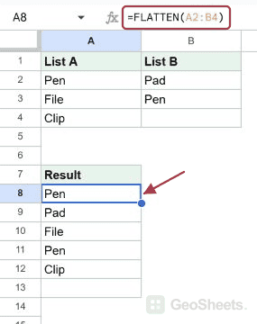
Below is the dataset, two columns of supplies where some items repeat across both columns.

Google Sheet with stationery items in 'Group A' and 'Group B', and a 'Unique Items' header.

You want a single deduplicated list of every distinct item.

Here is the formula:

=UNIQUE(FLATTEN(A2:B4))
Google Sheets with `=UNIQUE(FLATTEN(A2:B4))` in C2, showing unique flattened items.

FLATTEN collapses the 6-cell grid into one column of six values. UNIQUE then keeps only the first occurrence of each, leaving four distinct items in column C.

Pro Tip: UNIQUE wrapped around FLATTEN is one of the most common patterns. Use it whenever you need distinct values across a multi-column range.

Example 4: Turn a Single Row into a Column

FLATTEN also handles horizontal ranges. Pass it a row and the values come back as a column.

Below is the dataset, five quarterly totals laid out across row 2.

Google Sheets showing five quarter headers with numeric data, and an 'As Column' label.

You want those same numbers stacked vertically starting at F2.

Here is the formula:

=FLATTEN(A2:E2)
Google Sheets: FLATTEN(A2:E2) in F2 converts the row data into a vertical list.

FLATTEN reads A2 through E2 left-to-right and writes them down column F. If you only need to swap rows and columns rather than fully flatten, reach for TRANSPOSE; if you want to flatten, FLATTEN is the cleaner option.

Tips & Common Mistakes

  • Reading order matters. FLATTEN goes row by row, not column by column. For a column-first stack, transpose first or use VSTACK on the columns.
  • Blanks come through. Empty cells in the source range become empty entries in the spill. Wrap with FILTER if you need to drop them.
  • Mixed types are fine. FLATTEN happily mixes numbers and text in one column, which makes it a handy feeder for COUNTUNIQUE across irregular ranges.

FLATTEN is one of those small functions that quietly becomes essential once you start chaining it into bigger formulas. Use it any time you need a 2D range collapsed into a single column for the next step.

List of All Google Sheets Functions

Related Google Sheets Functions / Articles: