
CHOOSECOLS creates a new array containing the columns you select. Give it a range and column positions, listed in the order you want them to appear. The source table stays unchanged.
CHOOSECOLS function syntax
=CHOOSECOLS(array, col_num1, [col_num2, ...])- array: the source range or array.
- col_num1 and additional positions: 1 is the first column of that range, 2 is the second, and so on.
- Negative positions count from the right. -1 means the last column in the supplied range.
Set up the example data
Enter this dataset starting in A1. The first row contains headings. Keep the result area separate from the source table.
| Item | Category | Price | Units |
|---|---|---|---|
| Apple | Fruit | 2 | 120 |
| Bread | Bakery | 4 | 80 |
| Cheese | Dairy | 6 | 150 |
Extract one column
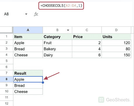
Enter this formula in A8. Column 1 of A2:D4 is the Item column, so the three item names expand into A8:A10. The source heading is excluded.
=CHOOSECOLS(A2:D4,1)Result: Apple; Bread; Cheese.
Reorder the selected columns
List position 3 before position 1 to return Price followed by Item. You can select nonadjacent columns without copying or rearranging the source.
=CHOOSECOLS(A2:D4,3,1)Result: 2, Apple; 4, Bread; 6, Cheese.
Select the last column from the right
The last column of A2:D4 is Units, so -1 returns 120, 80 and 150. Use -2 for Price, the second column from the right.
=CHOOSECOLS(A2:D4,-1)Result: 120; 80; 150.
Repeat a column when building an output
A position may appear more than once. This repeats Item twice and then adds Price. The result has three columns even though only two distinct source columns are used.
=CHOOSECOLS(A2:D4,1,1,3)Result: Apple, Apple, 2; Bread, Bread, 4; Cheese, Cheese, 6.
Filter rows and then choose columns
FILTER keeps Apple and Cheese because their units exceed 100. CHOOSECOLS then returns the first and third columns of that filtered array: Item and Price.
=CHOOSECOLS(FILTER(A2:D4,D2:D4>100),1,3)Result: Apple, 2; Cheese, 6.
Keep headings when they belong in the output
Starting the source at row 1 includes the heading row. This result returns Item and Price with their headers, followed by the three data rows.
=CHOOSECOLS(A1:D4,1,3)Result: Item, Price; Apple, 2; Bread, 4; Cheese, 6.
Handle a filter with no matching rows
Choose the columns first, then let FILTER apply the row condition. IFNA now handles the no-match result from FILTER directly. With the threshold raised to 999, this returns the fallback message.
=IFNA(FILTER(CHOOSECOLS(A2:D4,1,3),D2:D4>999),"No matching rows")Result: No matching rows.
Other Google Sheets articles you may also like