
If you have the year, month, and day sitting in separate cells and want to turn them into a single real date, the DATE function in Google Sheets is what you need.
It takes three numbers and builds a proper date you can sort, filter, and do math with. In this article I’ll show you how to use it with four practical examples.
DATE Function Syntax in Google Sheets
Here is how you write the DATE function.
=DATE(year, month, day)
- year – the year for the date, like 2024. A four-digit year is safest.
- month – the month number, where 1 is January and 12 is December.
- day – the day of the month, from 1 to 31.
When to Use DATE Function
- Combine separate year, month, and day columns into one usable date.
- Build a date from numbers your other formulas produce, like YEAR or MONTH results.
- Shift a date forward or back by adding to the year, month, or day argument.
- Create a fixed start or end date inside a larger formula without typing it as text.
Example 1: Build a Date From Year, Month, and Day
Let’s start with the core job, joining three columns into one date.
Below is the dataset, with the Year in column A, the Month in column B, and the Day in column C, across rows 2 to 6.
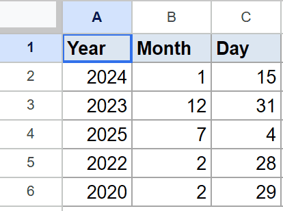
The goal is to take each row’s three numbers and turn them into a single date in column D.
Here is the formula:
=DATE(A2,B2,C2)
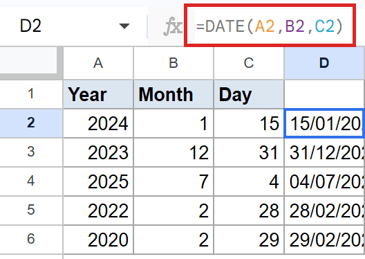
DATE reads the three numbers in order and stitches them together. So 2024, 1, and 15 becomes January 15, 2024.
Google Sheets stores that as a date and shows it formatted in the cell. The last row, 2020 with month 2 and day 29, becomes February 29, 2020, a valid leap day.
Pro Tip: Instead of filling the formula down row by row, you can build the whole column with one formula: =ARRAYFORMULA(DATE(A2:A6,B2:B6,C2:C6)). Same result, just one cell to manage.
Example 2: Month Values That Roll Into the Next Year
Here is a handy trick that surprises people the first time they see it.
Below is the dataset, again with Year, Month, and Day in columns A, B, and C. This time some of the month values are outside the normal 1 to 12 range.
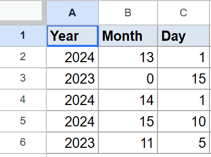
The goal is to see what DATE does when the month is something like 13 or 0.
Here is the formula:
=DATE(A2,B2,C2)
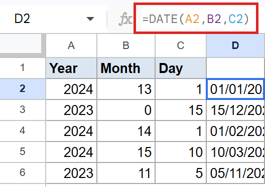
DATE does not throw an error when the month is out of range. It rolls the extra months into the neighboring year instead.
Month 13 of 2024 becomes January 1, 2025, since 13 is one month past December. Month 0 of 2023 rolls back to December 1, 2022, because 0 sits one month before January.
This is useful when a calculation hands you a month number that drifts past 12 or below 1. You don’t have to clean it up first.
Example 3: Day Values That Spill Into the Next Month
The same roll-over logic applies to the day argument too.
Below is the dataset, with Year, Month, and Day in columns A, B, and C. The day values here run past the end of the month on purpose.
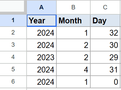
The goal is to watch how DATE handles a day number that the month can’t hold.
Here is the formula:
=DATE(A2,B2,C2)
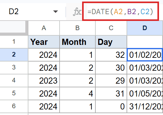
January only has 31 days, so day 32 of January 2024 rolls forward to February 1, 2024. The leftover day spills into the next month.
The same thing happens with February. Day 30 of February 2024 becomes March 1, 2024. A day of 0 rolls back to the last day of the previous month, so January 0 of 2024 lands on December 31, 2023.
Example 4: Add One Year to an Existing Date
You can do math right inside the arguments, which makes shifting a date easy.
Below is the dataset, with the original Year, Month, and Day in columns A, B, and C.
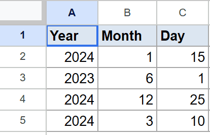
The goal is to push each date forward by exactly one year.
Here is the formula:
=DATE(A2+1,B2,C2)
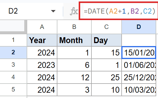
Adding 1 to the year argument is all it takes. The month and day stay the same, so the date just moves up a year.
The first row, originally 2024, January, 15, becomes January 15, 2025. You could use the same trick on the month or day argument to step a date forward by months or days instead.
Tips & Common Mistakes
- Use a full four-digit year. A two-digit year like 24 is read as the year 24, not 2024, which throws your dates off by centuries.
- Out-of-range months and days do not error out. They roll into the neighboring period, which is handy but can surprise you if you expected an error.
- If the result shows a plain number instead of a date, the cell is formatted as a number. Change the cell format to Date and it displays correctly.
DATE is the cleanest way to turn loose numbers into a real date your sheet can work with. Once the result is a true date, sorting, filtering, and date math all just work.
Try it on your own year, month, and day columns and see how much tidier your dates become.
List of All Google Sheets Functions
Related Google Sheets Functions / Articles: