
If you want to check whether at least one of several conditions is true, the OR function in Google Sheets is what you reach for. It looks at every condition you give it and returns TRUE the moment any one of them passes.
In this article, I’ll show you how to use OR with numbers, text, inside an IF, and across a whole range of values.
OR Function Syntax in Google Sheets
The OR function takes one or more conditions and returns a single TRUE or FALSE.
=OR(logical_expression1, [logical_expression2, ...])
- logical_expression1 is the first condition to test. It can be a comparison, a cell reference, or a range that resolves to TRUE/FALSE values.
- logical_expression2, … are optional extra conditions. You can keep adding more, separated by commas.
When to Use OR Function
- Flag a row when any one of several conditions is met, like passing if either score clears the bar.
- Check a single cell against a list of accepted text values at once.
- Combine OR with the IF function to return a readable label instead of TRUE or FALSE.
- Test a whole column of TRUE/FALSE checks to see if at least one passed.
Example 1: Pass If Either Subject Clears 40
Let’s start with the classic case, where a row passes if any single condition is true.
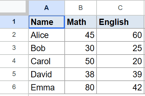
Below is the dataset. Column A has the student name, column B has the Math score, and column C has the English score.
I want to mark a student as passing if either subject is 40 or higher.
Here is the formula:
=OR(B2>=40, C2>=40)
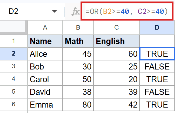
OR checks both conditions and returns TRUE if either one is met. For Alice, Math is 45, so the first condition passes and the result is TRUE. For Bob, both scores sit below 40, so the result is FALSE.
The formula in D2 is filled down so every student gets their own check.
Pro Tip: If you’d rather use one formula instead of filling down, wrap the check in ARRAYFORMULA: =ARRAYFORMULA(OR(B2:B6>=40, C2:C6>=40)). Note that this returns one combined answer for the whole range, so for a per-row result keep the fill-down version.
Example 2: Flag Specific Order Statuses
Here OR checks one cell against more than one text value.
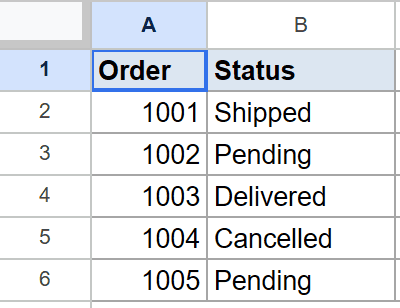
Below is the dataset. Column A has the order number and column B has the order status.
I want to flag any order that is either Pending or Cancelled.
Here is the formula:
=OR(B2="Pending", B2="Cancelled")
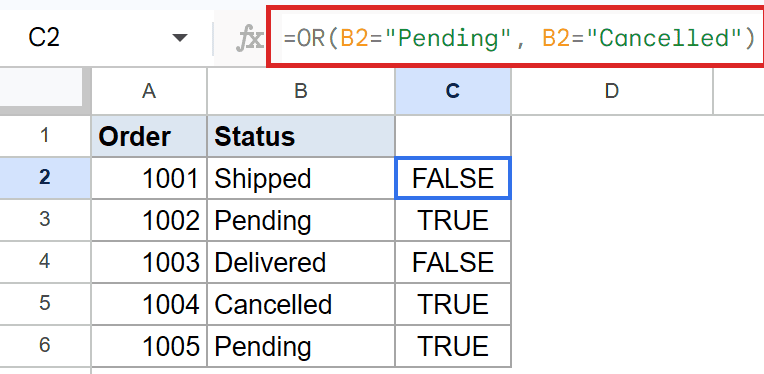
Each condition compares the status cell to one text value. Order 1001 is Shipped, so neither condition matches and the result is FALSE. Order 1002 is Pending, so the first condition matches and the result is TRUE.
This is handy when you want one flag column for several statuses without writing a long nested formula.
Example 3: OR Inside an IF
OR on its own returns TRUE or FALSE, which isn’t always the friendliest output. Wrapping it in an IF fixes that.
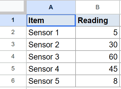
Below is the dataset. Column A has the sensor name and column B has its reading.
I want to show “Check” when a reading is out of range, meaning below 10 or above 50, and “OK” otherwise.
Here is the formula:
=IF(OR(B2<10, B2>50), "Check", "OK")
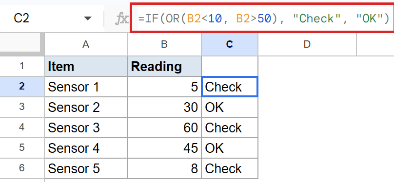
The OR runs first and hands its TRUE/FALSE answer to the IF function, which then picks the label. Sensor 1 reads 5, which is below 10, so OR is TRUE and the result is “Check”. Sensor 2 reads 30, which sits inside the range, so OR is FALSE and the result is “OK”.
This pattern is the most common way people use OR in real sheets, since a plain TRUE/FALSE rarely reads well in a report.
Example 4: OR Across a Range of Checks
OR can also take a whole range at once instead of separate conditions.
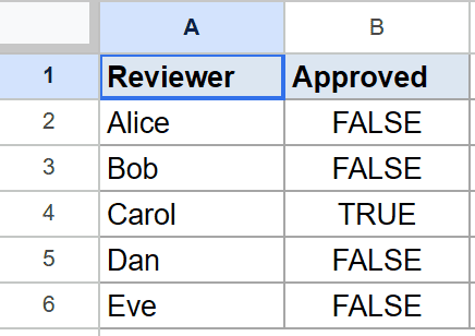
Below is the dataset. Column A has the reviewer name and column B has a TRUE/FALSE approval value for each one.
I want to know if at least one reviewer has approved.
Here is the formula:
=OR(B2:B6)
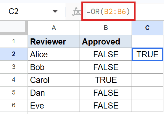
When you feed OR a range, it scans every value in it. Most reviewers here are FALSE, but Carol is TRUE, so the formula returns TRUE. Only if every single value were FALSE would the result come back FALSE.
This is the quick way to ask “did anyone say yes?” across a column without listing each cell by hand.
Tips & Common Mistakes
- OR returns TRUE if any condition passes, not all of them. If you actually need every condition to be true, use AND instead. Mixing the two up is the most common OR mistake.
- Wrap text values in double quotes. A condition like B2=”Pending” only works with the quotes around the text. Without them, Sheets treats Pending as a named range and the formula breaks.
- A range argument like OR(B2:B6) returns one answer, not one per row. If you want a separate result for each row, give OR the per-row conditions and fill the formula down, as in the first three examples.
OR is the function for “at least one of these is true” logic.
You’ve now seen it with numbers, text, inside an IF, and across a full range. Pick the form that matches whether you need a per-row answer or a single combined one.
List of All Google Sheets Functions
Related Google Sheets Functions / Articles: