
IFS returns the value associated with the first true condition. List each condition immediately before its result, and order overlapping conditions so the intended match comes first.
IFS function syntax
=IFS(condition1, value1, [condition2, value2, ...])- condition1: a logical test such as A2>=90.
- value1: the result associated with that test.
- Additional conditions and values come in pairs.
- If no condition is true, the result is #N/A. A final TRUE condition can provide a fallback.
Set up the example data
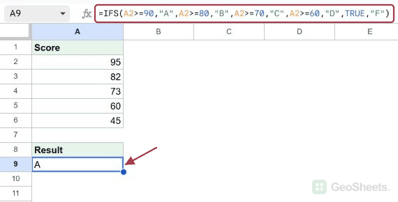
Enter this dataset starting in A1. The first row contains headings. Keep the result area separate from the source table.
| Score |
|---|
| 95 |
| 82 |
| 73 |
| 60 |
| 45 |
Assign a letter grade
Enter this formula in A9. A score of 95 qualifies for several lower thresholds, but the >=90 test comes first, so IFS returns A.
=IFS(A2>=90,"A",A2>=80,"B",A2>=70,"C",A2>=60,"D",TRUE,"F")Result: A.
Describe temperatures with explicit units
This example uses degrees Fahrenheit. A reading of 72 returns Comfortable under the chosen bands. The labels are illustrative comfort categories, not a medical or safety rule.
=IFS(72>=90,"Too hot",72>=60,"Comfortable",72>=32,"Cold",TRUE,"Below freezing")Result: Comfortable.
Classify order quantities
For 100 orders, the first test is true and the result is High. Exactly 10 is Medium; values below 10 fall to Low. Set the thresholds to your reporting rules.
=IFS(100>=100,"High",100>=10,"Medium",TRUE,"Low")Result: High.
Return a numeric commission rate
For illustrative sales of 8000, this returns 0.1, a numeric 10% rate. Apply percentage formatting to the result. The rate can then be multiplied by sales without relying on conversion from text.
=IFS(8000>=10000,15%,8000>=7000,10%,8000>=4000,5%,TRUE,0%)Result: 0.1.
Use ascending upper bounds for age bands
For age 19, the <13 condition fails and <20 succeeds, returning Teen. With less-than thresholds, test the smallest upper limit first. These are illustrative labels, not eligibility rules.
=IFS(19<13,"Child",19<20,"Teen",19<65,"Adult",TRUE,"Senior")Result: Teen.
Leave a missing input unclassified
A7 is blank in this dataset. An outer IF returns empty text before the grade logic runs. This prevents a missing score from automatically receiving the lowest grade.
=IF(A7="","",IFS(A7>=90,"A",A7>=80,"B",TRUE,"Below B"))Result: empty text, displayed as a blank cell.
Decide whether unmatched input should be visible
Here no condition is true, so #N/A is returned. Add a final TRUE and a message only when a fallback is part of your intended rule. It is not mandatory for every IFS formula.
=IFS(45>=90,"A",45>=80,"B")Result: #N/A.
Other Google Sheets articles you may also like