SWITCH Function in Google Sheets

If you want a clean way to translate one value into another, like turning a code into a label or a number into a category, the SWITCH function in Google Sheets handles it without the long IF chain. You give it an expression and a list of case-then-result pairs. It returns the result for the first match.

In this article, I’ll show you how to use SWITCH to map text codes and translate numeric codes. I’ll also cover how to switch on an expression, how to mimic IFS-style boolean cases, and how to apply a different calculation per category.

SWITCH Function Syntax in Google Sheets

The SWITCH function returns a value based on the first matching case from a list.

=SWITCH(expression, case1, value1, [case2, value2, ...], [default])
  • expression is the value or formula you want to test, like a cell reference or MOD(A2,2).
  • case1 is the first value to compare against the expression.
  • value1 is the result returned if case1 matches.
  • case2, value2, … are optional extra case-value pairs.
  • default is the optional fallback returned when nothing matches.

SWITCH is a compact alternative to a long nested IF chain when the job is “look up a value, return a value”. It also overlaps with the CHOOSE function, but CHOOSE keys off a position index while SWITCH matches the actual value.

When to Use SWITCH Function

  • Convert a code into a readable label, like turning “M” into “Monday” or 1 into “Electronics”.
  • Translate a category or tier number into a name without nesting IFs.
  • Apply a different calculation depending on a category, like a region-specific commission rate.
  • Replace a tall IFS chain when you’re comparing the same input against multiple constant values.
  • Switch on an expression like MOD or LEFT, not just a single cell reference.

Example 1: Map Day Codes to Weekday Names

Let’s start with the most common use, turning a single-letter code into a full weekday name.

Below is the dataset. Column A has the single-letter code for each day, and column B is where the weekday name will land.

Google Sheets dataset: 'Code' column has M, T, W, R, X; 'Day' column is empty.

I want to convert each code into the full weekday name, with a fallback of “Unknown” for anything that doesn’t match.

Here is the formula:

=SWITCH(A2, "M", "Monday", "T", "Tuesday", "W", "Wednesday", "R", "Thursday", "F", "Friday", "Unknown")
Google Sheets SWITCH function in B2 maps codes to days, including an 'Unknown' default.

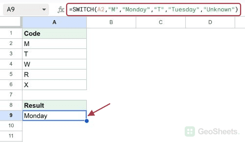
SWITCH checks A2 against each case in order. “M” matches first for row 2, so the result is “Monday”. The same logic plays out for T, W, and R, returning Tuesday, Wednesday, and Thursday.

The last row has an “X” code, which matches none of the cases. SWITCH falls back to the final argument, “Unknown”, and returns that.

Pro Tip: The default value is whatever you put as the last argument after all the case-value pairs. Leave it out and SWITCH returns an #N/A error when nothing matches.

Example 2: Numeric Code to Product Category

SWITCH works with numeric cases too, not just text.

Below is the dataset. Column A has a numeric category code and column B is where the category name will appear.

Dataset for SWITCH function: 'Code' column with numbers, 'Category' column is blank.

I want to translate each code into a readable category name, with “Other” as the fallback for any unrecognized code.

Here is the formula:

=SWITCH(A2, 1, "Electronics", 2, "Clothing", 3, "Books", 4, "Home", "Other")
Google Sheets: Cell B2 displays a SWITCH formula, mapping codes to categories.

Each numeric code maps to its label. Row 2 holds 1 and returns “Electronics”, row 3 holds 3 and returns “Books”, and so on.

The row with code 5 doesn’t match any case, so it falls through to “Other”. This is a much cleaner way to handle this kind of mapping than a nested IF chain would be.

Example 3: Switch on an Expression Like MOD

The first argument to SWITCH doesn’t have to be a plain cell reference. It can be an expression.

Below is the dataset. Column A has a number and column B is where the parity label will land.

Google Sheet showing Number column (4, 7, 10, 13, 22) and an empty Parity column.

I want to label each number as “Even” or “Odd” based on whether dividing it by 2 leaves a remainder.

Here is the formula:

=SWITCH(MOD(A2,2), 0, "Even", 1, "Odd")
Google Sheets: B2 'Even' is result of SWITCH function checking A2's number parity.

MOD(A2,2) returns the remainder when A2 is divided by 2. SWITCH then matches that remainder against 0 or 1.

Rows with 4, 10, and 22 leave a remainder of zero and get labeled “Even”. The rows with 7 and 13 leave a remainder of one and get labeled “Odd”. Whatever you can compute, you can switch on.

Example 4: Use TRUE to Mimic IFS-Style Cases

This is the SWITCH power-user trick. By passing TRUE as the expression, each case becomes a boolean test instead of an equality check.

Below is the dataset. Column A has a numeric score and column B is where the letter grade will appear.

Google Sheets with "Score" column (95, 82, 73, 64, 55) and empty "Grade" column.

I want to assign a letter grade based on score thresholds, like 90 and above for A, 80 to 89 for B, and so on.

Here is the formula:

=SWITCH(TRUE, A2>=90, "A", A2>=80, "B", A2>=70, "C", "F")
Google Sheets: SWITCH formula in B2 maps scores to grades, with 95 as 'A'.

SWITCH compares TRUE to each case in order. Each case is now a boolean expression like A2>=90, which itself returns TRUE or FALSE. The first case that evaluates to TRUE wins.

A score of 95 makes A2>=90 true, so the result is “A”. A score of 82 fails the first test but passes A2>=80, returning “B”. The 73 row passes only the A2>=70 test, landing on “C”. Scores below 70 fall through to the “F” default.

This is basically the same job that the IFS function does for boolean conditions. SWITCH(TRUE, …) is just an alternative spelling.

Pro Tip: Order matters with the TRUE trick. SWITCH stops at the first TRUE case, so put your strictest test first. A score of 95 passes both `>=90` and `>=80`, but `>=90` comes first, so the result is “A”.

Example 5: Different Commission Rate per Region

Each case in SWITCH can return a formula, not just a constant. This lets you apply a different calculation per category.

Below is the dataset. Column A has the region, column B has the sale amount, and column C is where the calculated commission will land.

Google Sheet showing Region and Sales data, with an empty Commission column.

I want to apply a different commission rate to the sale amount depending on the region, with a fallback rate for anything else.

Here is the formula:

=SWITCH(A2, "East", B2*0.1, "West", B2*0.08, "North", B2*0.06, B2*0.05)
C2 in Google Sheets displays a SWITCH formula calculating commission by region with varied rates.

For each region, SWITCH picks the matching multiplier and applies it to the sale amount. East gets 10 percent, West gets 8 percent, North gets 6 percent, and anything else falls back to 5 percent.

Row 2 has East with 1000 in sales, so the commission is 100. Row 3 has West with 2000, returning 160. The South row falls through to the 5 percent fallback, applying it to 1500 to give 75.

Putting a formula on the result side of each case turns SWITCH into a tidy way to handle calculation rules that change by category.

Tips & Common Mistakes

  • The default is optional but worth adding. Without a default value, SWITCH returns #N/A when no case matches. Add a final argument like “Other” or 0 to handle the unknowns.
  • SWITCH only does equality checks. Cases get compared with equals, not with operators like greater than. To get range-based logic, use the SWITCH(TRUE, …) trick from Example 4, or use the IFS function instead.
  • Mind the case order. SWITCH returns the result of the first matching case and stops. If two cases could match, the order you list them in decides the outcome. The TRUE-style pattern is the most common place this trips people up.

SWITCH is a clean way to map a value to another value when the input matches one of a known set of cases.

You’ve now seen it with text codes, numeric codes, a MOD expression, the TRUE-style boolean trick, and a per-category calculation. Use it whenever a nested IF chain feels heavier than the job calls for.

List of All Google Sheets Functions

Related Google Sheets Functions / Articles: