If you want to pick a value from a list of options based on a number, the CHOOSE function in Google Sheets is the simplest way to do it.
You pass it an index and a list, and it returns the item at that position.
In this article, I’ll walk you through five practical examples that show CHOOSE in action, including status labels, picking between calculations, commission tiers, weekday names, and even returning an entire range to sum.
CHOOSE Function Syntax in Google Sheets
CHOOSE takes an index followed by the list of values to pick from.
=CHOOSE(index, choice1, [choice2, ...])
index: a number from 1 up to the number of choices. 1 picks the first choice, 2 picks the second, and so on.choice1: the value returned when index is 1. Can be a number, a text string, a cell reference, or a range.choice2, ...(optional): additional choices. You can list up to 30 choices.
CHOOSE indexes start at 1, not 0. If the index is below 1 or above the number of choices, CHOOSE returns a #VALUE! error.
When to Use CHOOSE Function
- Turn a numeric code into a readable label without nesting a long chain of IF statements.
- Switch between different calculations or formulas based on a mode input.
- Map a tier or category number to a rate, multiplier, or factor.
- Convert a weekday or month number into its short name.
- Pick which range to feed into another function such as SUM or AVERAGE.
Example 1: Pick a status label by its index number
Let’s start with the basic case. You have a column of status codes from 1 to 4 and you want to convert each one into a readable label.
Below is a small table with status codes in column A.
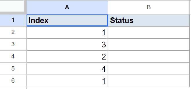
The goal is to return the matching status text next to each index number.
Here is the formula:
=CHOOSE(A2,"Pending","Approved","Shipped","Delivered")
Put it in B2 and fill it down through B6.
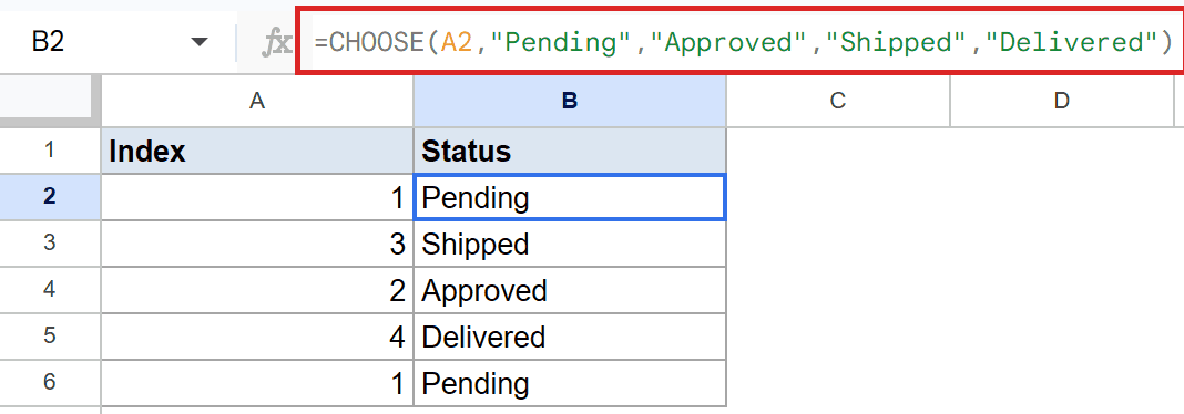
B2 returns Pending since the index is 1, B3 returns Shipped (index 3), B4 returns Approved (index 2), B5 returns Delivered (index 4), and B6 returns Pending again.
CHOOSE just reads the index in column A and hands back the matching item from the list of four labels.
Pro Tip: If you’d rather use a single formula instead of filling down, wrap CHOOSE in ARRAYFORMULA: =ARRAYFORMULA(CHOOSE(A2:A6,"Pending","Approved","Shipped","Delivered")). The result spills into the same five cells.
Example 2: Switch between calculations using a mode number
CHOOSE is not limited to returning text. It can return entire expressions, which means you can use it to pick which calculation to run.
Below is a table with two numbers and a mode column where 1 means add, 2 means subtract, 3 means multiply, and 4 means divide.
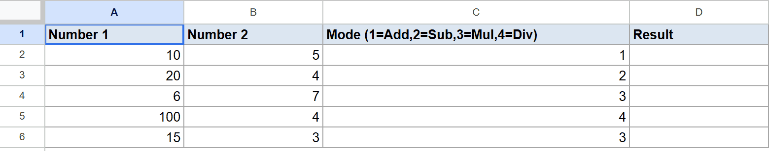
The goal is to run the right arithmetic operation on each row based on the mode in column C.
Here is the formula:
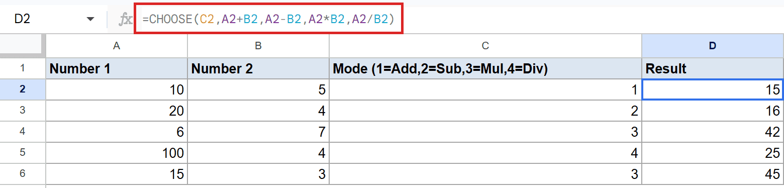
=CHOOSE(C2,A2+B2,A2-B2,A2*B2,A2/B2)
Put it in D2 and fill it down through D6.
How this formula works:
- The mode value in C2 is the index. CHOOSE uses it to pick one of the four expressions.
- All four expressions are calculated values, not text, so the result is a real number.
- Row 1 has mode 1, so CHOOSE returns
A2+B2, which is10+5=15. - Row 2 has mode 2, so it returns
20-4=16. Row 3 multiplies to 42, row 4 divides to 25, and row 5 multiplies again to 45.
Pro Tip: This pattern is a clean alternative to a nested IF chain. With four modes, an IF version would need three nested IFs. CHOOSE keeps it on one line and stays readable.
Example 3: Look up a commission rate by tier number
CHOOSE works nicely as a small lookup table when the keys are sequential integers. Here we use it to map a tier number to a commission rate, then multiply by the sales figure.
Below is a table of salespeople with their tier and sales numbers.
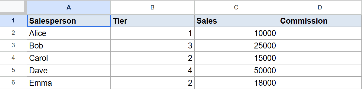
The goal is to calculate each person’s commission based on their tier.
Here is the formula:
=C2*CHOOSE(B2,0.05,0.08,0.1,0.15)
Put it in D2 and fill it down through D6.
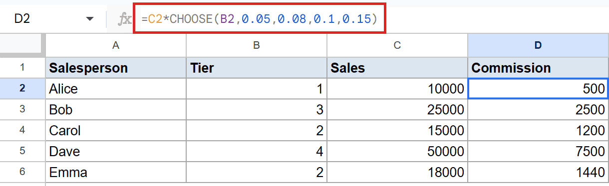
CHOOSE turns the tier number in column B into the matching commission rate. Tier 1 returns 5%, tier 2 returns 8%, tier 3 returns 10%, and tier 4 returns 15%.
Multiplying that rate by the sales value in column C gives the commission amount. Alice (tier 1, sales 10,000) earns 500, Bob (tier 3, sales 25,000) earns 2,500, and so on.
Pro Tip: For a small set of sequential tiers like this, CHOOSE is concise. If your tiers ever become non-sequential or you need lookup keys that aren’t simple integers, VLOOKUP or XLOOKUP against a rate table is a better fit.
Example 4: Convert a weekday number into a day name
The classic CHOOSE pairing is with WEEKDAY. WEEKDAY returns a number from 1 to 7 for a given date, and CHOOSE turns that number into a short day name.
Below is a table with five dates in early January 2026.
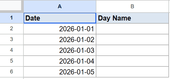
The goal is to show the short day name next to each date.
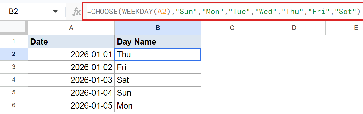
Here is the formula:
=CHOOSE(WEEKDAY(A2),"Sun","Mon","Tue","Wed","Thu","Fri","Sat")
Put it in B2 and fill it down through B6.
How this formula works:
WEEKDAY(A2)returns 1 for Sunday, 2 for Monday, all the way up to 7 for Saturday (this is the default mode).- CHOOSE takes that number and picks the matching short name from the seven-item list.
- January 1, 2026 is a Thursday, so WEEKDAY returns 5 and CHOOSE returns
Thu. The rest follow in order: Fri, Sat, Sun, Mon.
Pro Tip: You can also get the day name with =TEXT(A2,"ddd"). The CHOOSE version is handy when you want to use custom labels (for example, full names in another language, or “Weekday” and “Weekend” buckets instead of seven separate names).
Example 5: Pick which column range to sum based on a quarter number
This is the example that surprises most people. CHOOSE can return entire ranges, not just single values, which means you can hand the picked range straight to a function like SUM.
Below is a table of regional sales by quarter, with a quarter input in B6.
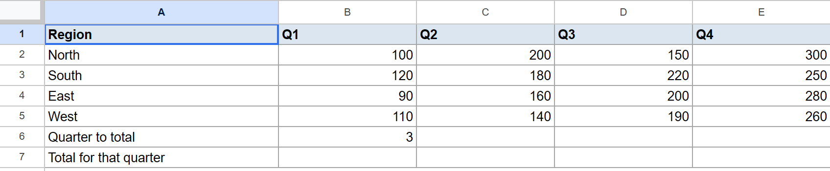
The goal is to total the chosen quarter’s sales across all four regions, controlled by the number in B6.
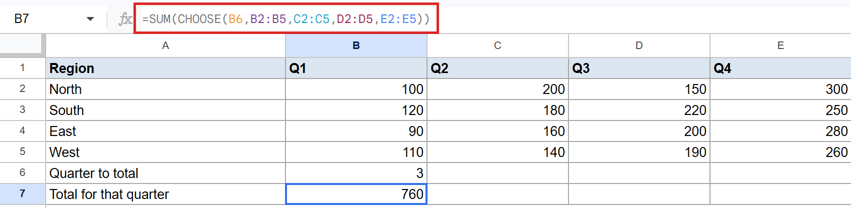
Here is the formula:
=SUM(CHOOSE(B6,B2:B5,C2:C5,D2:D5,E2:E5))
Put it in B7.
How this formula works:
- B6 holds the quarter number. In this case it’s 3, so CHOOSE picks the third range in the list, which is
D2:D5(the Q3 column). - That range goes straight into SUM, which adds up the four Q3 values: 150 + 220 + 200 + 190.
- The total is 760. Change B6 to 1, 2, or 4 and the formula re-points SUM at a different quarter’s column.
Pro Tip: This is one of CHOOSE’s most underrated capabilities. Most lookup functions return a single value. CHOOSE happily returns a whole range, which makes it a clean way to swap inputs into functions like SUM, AVERAGE, COUNT, or even another range-based function.
Tips & Common Mistakes
- CHOOSE indexes start at 1, not 0. If you’re coming from a programming background, the off-by-one is easy to miss.
=CHOOSE(0,"a","b")returns#VALUE!, not the first item. The first valid index is 1. - Out-of-range index returns an error. If your index is greater than the number of choices (for example,
=CHOOSE(5,"a","b","c")), CHOOSE returns#VALUE!. Make sure the input range is bounded, or wrap the formula in IFERROR to handle stray values. - For long lists, IFS or SWITCH may read cleaner. CHOOSE is at its best when you’re picking by a sequential integer 1, 2, 3. Once the keys are arbitrary or there are more than about ten items, IFS or SWITCH (or a lookup table with VLOOKUP) usually scales better.
CHOOSE looks simple, and it is, but the moment you realize it can return entire ranges and full expressions, it stops being a basic helper and starts being a real switching tool.
It’s the cleanest way to pick between calculations, ranges, or labels in a single readable line.
List of All Google Sheets Functions
Related Google Sheets Functions / Articles: