
VLOOKUP in Google Sheets searches the first column of a table and returns a value from the same row. Use FALSE as the final argument when you want an exact match.
Look Up an Exact Salary by Name
Enter this dataset starting in A1. Leave cells marked “(blank)” empty.
| Employee | Salary |
|---|---|
| Maya | 71000 |
| Noah | 64000 |
| Ari | 68000 |
| Lena | 75000 |
| Omar | 60000 |
Enter this formula in E2:
=VLOOKUP("Maya",$A$2:$B$6,2,FALSE)The result is 71000. VLOOKUP finds Maya in column A and returns her salary from the second column of the selected range. The table does not need sorting for this exact match.
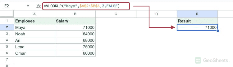
Replace "Maya" with a cell reference to make the lookup respond to another cell. Dollar signs lock the table when you copy the formula, while an unanchored search-cell reference can change by row.
VLOOKUP Function Syntax
=VLOOKUP(search_key, range, index, [is_sorted])| Argument | Purpose |
|---|---|
| search_key | Value to find in the first column |
| range | Lookup table, including the return column |
| index | Return column position within that range, starting at 1 |
| is_sorted | FALSE for exact; TRUE or omitted for approximate |
Specify FALSE for exact matching. Omitting the last argument selects approximate matching. That can silently return an unintended row when the lookup column is unsorted.
The column index is relative to your range. If the range starts in C, index 2 means column D. An index beyond the range width returns #REF!.
Use Approximate Matching for Grade Bands
Enter this dataset starting in A12. Leave cells marked “(blank)” empty.
| Minimum score | Grade |
|---|---|
| 0 | F |
| 60 | D |
| 70 | C |
| 80 | B |
| 90 | A |
=VLOOKUP(76,A13:B17,2,TRUE)The score 76 returns C, using the threshold 70. Approximate matching chooses the largest threshold at or below the score. The threshold column must be sorted ascending, with each grade kept beside its threshold.
A score below the smallest threshold returns #N/A. Use this method for deliberate bands such as grades or pricing tiers, rather than IDs that must match exactly.
Return a Column Further Right
Enter this dataset starting in A23. Leave cells marked “(blank)” empty.
| ID | Product | Price | Stock |
|---|---|---|---|
| P01 | Pen | 2 | 58 |
| P02 | Paper | 5 | 0 |
| P03 | Folder | 3 | 21 |
=VLOOKUP("P01",A24:D26,4,FALSE)The result is 58, from the Stock column. Looking up P02 returns 0, which is a real stock value. VLOOKUP searches the first column of the supplied table, even when returning a later column.
For a return column to the left of the key, XLOOKUP or INDEX with MATCH is usually clearer. VLOOKUP cannot use a negative column index to look left.
Handle Missing Values with IFNA or IFERROR
=IFNA(VLOOKUP("Missing",A2:B6,2,FALSE),"Not found")This returns Not found for a lookup that produces #N/A. Check the spelling and data type of the key first: leading spaces or number-versus-text differences can cause an apparently valid key to miss.
The broader original pattern also works:
=IFERROR(VLOOKUP("Missing",A2:B6,2,FALSE),"Not found")IFERROR catches every error, including a broken column index. Its fallback therefore does not prove that the record is absent. Prefer IFNA when you want other formula errors to remain visible.
Choose the Return Column with MATCH
Enter this dataset starting in A33. Leave cells marked “(blank)” empty.
| Student | Math | Science | English |
|---|---|---|---|
| Maya | 88 | 95 | 90 |
| Noah | 80 | 85 | 82 |
| Ari | 92 | 89 | 91 |
=VLOOKUP("Maya",A34:D36,MATCH("Science",A33:D33,0),FALSE)The result is 95. MATCH locates Science in the header row and supplies its position as VLOOKUP’s column index. The headers and data range must start in the same column.
Handle Duplicate Names, Case, and Wildcards
Exact VLOOKUP is not case-sensitive: maya matches Maya. If the same key appears twice, it returns the first matching row. Use unique IDs when duplicate names could identify different people.
=VLOOKUP("M*",A2:B6,2,FALSE)The asterisk matches any sequence of characters, so this returns Maya’s 71000. A question mark matches one character. Wildcards work with FALSE, so “exact” mode can still support intentional pattern matching.
Look Up Data on Another Tab
=VLOOKUP("Maya",'GS30-VLOOKUP'!A2:B6,2,FALSE)This returns the same salary from the named tab. Replace the tab name with yours. For a different spreadsheet file, IMPORTRANGE imports the lookup table and requires the relevant access permission.
Other Google Sheets articles you may also like