HLOOKUP Function in Google Sheets

If you want to look up a value in the first row of a table and pull a matching value from a row below it, HLOOKUP is the function for that.

It’s the horizontal cousin of VLOOKUP, designed for cases where your data is laid out across rows instead of down columns.

In this article, I’ll walk you through five practical examples that cover exact matches, approximate matches, wildcards, and a two-way lookup combining HLOOKUP with MATCH.

HLOOKUP Function Syntax in Google Sheets

HLOOKUP takes up to four arguments.

=HLOOKUP(search_key, range, index, [is_sorted])

• search_key: the value to look up in the first row of the range.
• range: the lookup range. HLOOKUP searches the first row for search_key.
• index: the row number within the range whose value will be returned (1 = first row of the range).
• is_sorted (optional, default TRUE): FALSE for exact match (recommended); TRUE for approximate match against a sorted-ascending first row.

HLOOKUP is the horizontal sibling of VLOOKUP. VLOOKUP scans the first column of a range and returns a value from a column to the right. HLOOKUP scans the first row and returns a value from a row below.

When to Use HLOOKUP Function

• Pull a value from a table that’s laid out horizontally, with the lookup keys sitting in the top row.
• Translate a category or label (Q1, North, Tier A) into its matching value from a row beneath it.
• Build a grade or commission band lookup using the approximate-match mode against sorted breakpoints.
• Match partial text in the top row using ? and * wildcards in exact-match mode.
• Combine with MATCH to build a two-way lookup that picks both the column and the row dynamically.

Example 1: Basic exact-match HLOOKUP across a horizontal table

Let’s start with the simplest case. You have a single row of labels and a single row of values, and you want to pull the value for a given label.

Below is a small horizontal lookup table.

Row 1 holds quarter labels Q1 through Q5 in cells A1:E1, and row 2 holds the matching values 100 through 500 in A2:E2. Row 3 is left blank.

Row 4 has two headers, “Lookup Quarter” in A4 and “Result” in B4. Cells A5:A9 hold the quarters you want to look up, and column B is where the result will land.

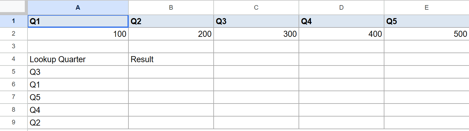
The goal is to look up each quarter from column A in the first row of the lookup table and return the matching value from row 2.

Here is the formula:

=HLOOKUP(A5, $A$1:$E$2, 2, FALSE)

Put it in B5 and fill it down through B9. The lookup range $A$1:$E$2 is locked with dollar signs so it stays put as the formula moves down.

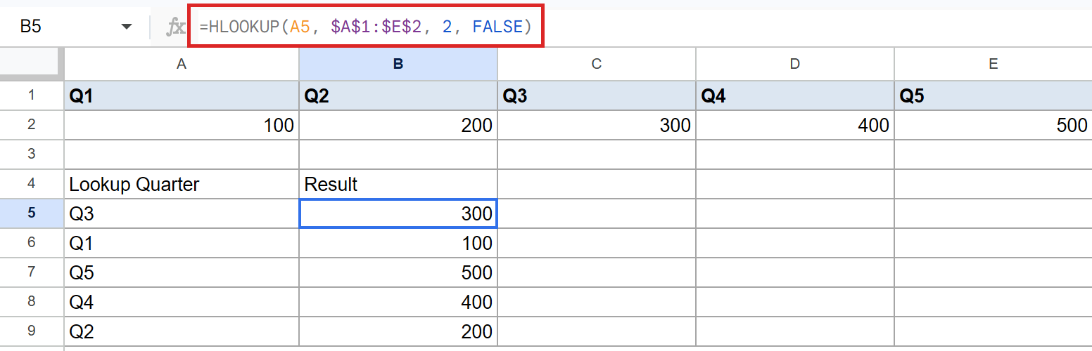
For B5, HLOOKUP looks for “Q3” in the first row of $A$1:$E$2, finds it in column C, and returns the value from row 2 of the range, which is 300.

The rest fill in the same way: 100 for Q1, 500 for Q5, 400 for Q4, and 200 for Q2. The fourth argument, FALSE, asks for an exact match, which is what you almost always want.

Pro Tip: The third argument, 2, is the row number inside the range, not the absolute sheet row. Since the range starts at row 1 of the sheet and only spans two rows, 2 means “the second row of the range,” which happens to also be sheet row 2. If your range started at row 3 of the sheet, 2 would refer to sheet row 4.

Example 2: Pull a value from a deeper row using a variable index

Sometimes the lookup table has more than two rows, and you want to pick which row to return on a per-lookup basis. The third argument can be driven by another cell.

Below is a four-region lookup table. Row 1 has the header “Quarter” in A1, then Q1, Q2, Q3, Q4 in B1:E1. Rows 2 through 5 hold the region names in column A (North, South, East, West) and their quarterly values in B2:E5. Row 6 is blank. Row 7 holds the headers “Lookup”, “Index”, and “Result” in A7:C7. Rows 8 through 11 hold the quarter to look up in column A and the index to return in column B.

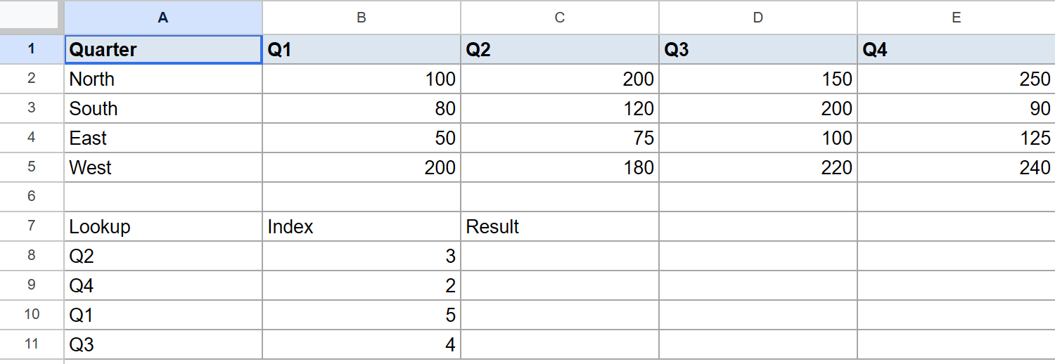
The goal is to look up each quarter in the first row of the numeric block and return the value from whichever row the index in column B points to.

Here is the formula:

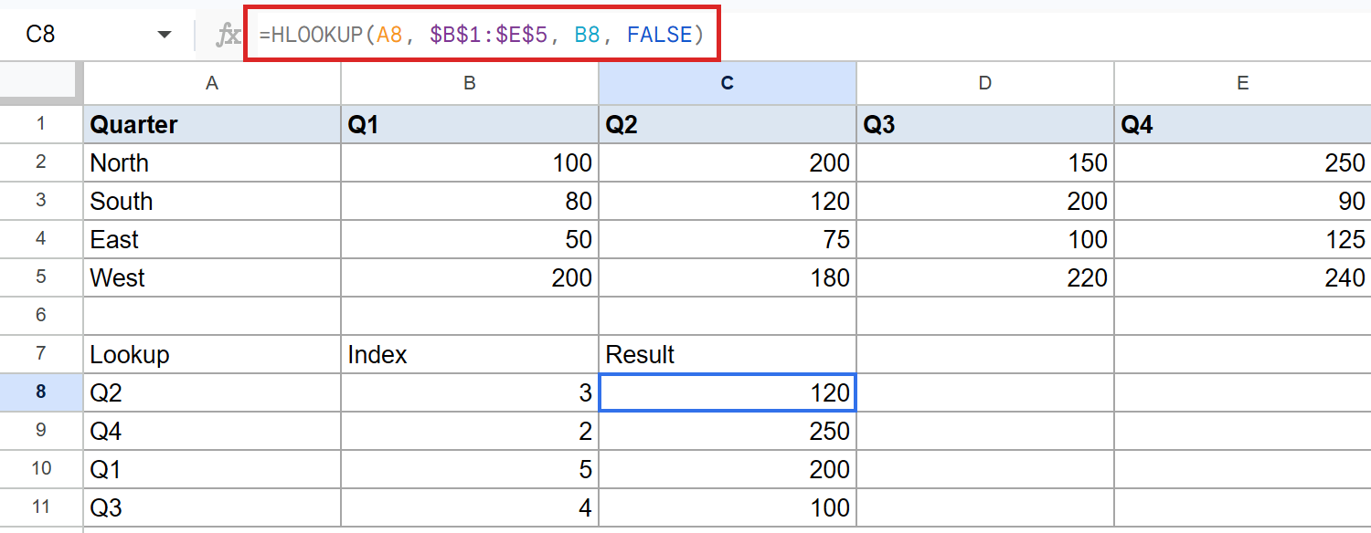
=HLOOKUP(A8, $B$1:$E$5, B8, FALSE)

Put it in C8 and fill it down through C11.

How this formula works:

• The lookup range is $B$1:$E$5, which is the numeric block only. The region labels in column A are excluded because HLOOKUP scans the first row of whatever range you give it, and you want Q1-Q4 there, not “Quarter”.
• A8 holds the quarter to find. For row 8, that’s Q2.
• B8 is the row index. For row 8, that’s 3, which means “the third row of the range.” Row 1 of the range is the header (Q1-Q4), row 2 is North, row 3 is South. So the result is South’s Q2 value, 120.
• The rest fill in the same way. Q4 with index 2 returns North’s Q4, which is 250. Q1 with index 5 returns West’s Q1, which is 200. Q3 with index 4 returns East’s Q3, which is 100.

Pro Tip: This pattern is the textbook reason HLOOKUP exists. With a single formula filled down, you can pull a different cell from a 2D table for every row of inputs.

Example 3: Approximate-match HLOOKUP for tiered lookups

The is_sorted argument flips HLOOKUP from exact match to approximate match. With TRUE, it finds the largest value in the first row that’s less than or equal to your search key. The first row must be sorted in ascending order for this to work correctly.

Below is a grade band. Row 1 has the breakpoints 0, 50, 100, 200, 500 in A1:E1, sorted ascending. Row 2 has the matching grades F, D, C, B, A in A2:E2. Row 3 is blank. Row 4 has the headers “Score” and “Grade” in A4 and B4. Rows 5 through 9 hold scores in column A.

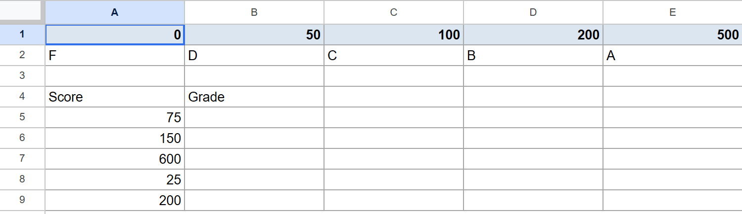
The goal is to convert each score into its matching grade band.

Here is the formula:

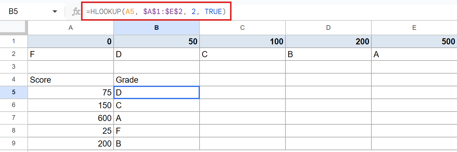
=HLOOKUP(A5, $A$1:$E$2, 2, TRUE)

Put it in B5 and fill it down through B9. Notice the fourth argument is TRUE this time.

How this formula works:

• For a score of 75, HLOOKUP scans the first row left to right looking for the largest breakpoint that’s less than or equal to 75. The breakpoints are 0, 50, 100, 200, 500. The largest one that’s not greater than 75 is 50, sitting in column B. So HLOOKUP returns the grade in row 2, column B, which is “D”.
• Score 150 finds breakpoint 100, returning “C”.
• Score 600 finds breakpoint 500, returning “A”.
• Score 25 finds breakpoint 0, returning “F”.
• Score 200 finds breakpoint 200 exactly, returning “B”.

Pro Tip: Approximate match only makes sense when your first row is genuinely sorted ascending and represents tier boundaries. If the row holds unsorted category labels (Q1, Q2, Q3…), use FALSE for exact match. Forgetting to pass FALSE on an exact-match lookup is one of the most common HLOOKUP mistakes, because the default behavior is TRUE.

Example 4: Match product codes using wildcards in HLOOKUP

In exact-match mode, HLOOKUP supports two wildcards. ? matches any single character, and * matches any sequence of characters. Useful when you only know part of the lookup key.

Below is a horizontal product table. Row 1 holds the codes “ABC123”, “XYZ456”, “DEF789”, “GHI012”, “JKL345” in A1:E1. Row 2 holds the prices 100 through 500 in A2:E2. Row 3 is blank. Row 4 has “Search Pattern” and “Price” headers in A4 and B4. Rows 5 through 8 hold wildcard patterns in column A.

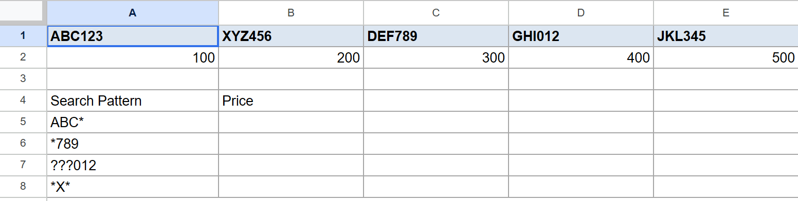
The goal is to use wildcard patterns to find the matching product and pull its price.

Here is the formula:

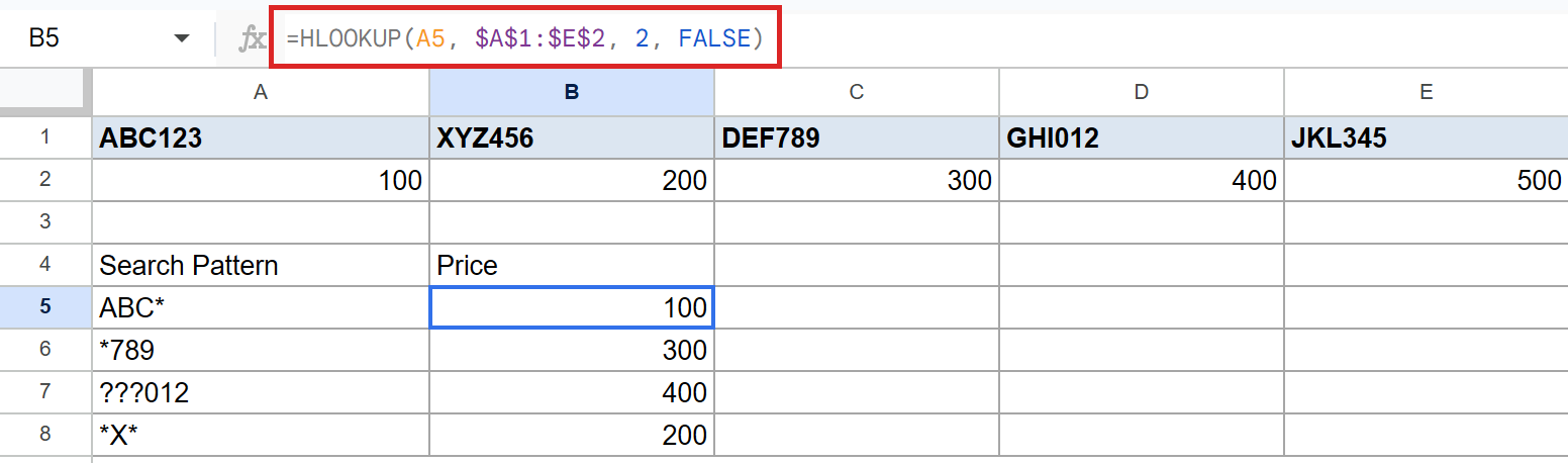
=HLOOKUP(A5, $A$1:$E$2, 2, FALSE)

Put it in B5 and fill it down through B8. The formula is identical to Example 1. The wildcards live in the search keys themselves, not in the formula.

How each pattern matches:

• ABC* matches “ABC123” (the * covers “123”), returning 100.
• *789 matches “DEF789” (the * covers “DEF”), returning 300.
• ???012 uses three ? wildcards to match exactly three characters followed by “012”, landing on “GHI012”, returning 400.
• *X* matches anything containing an X, which is “XYZ456”, returning 200.

Pro Tip: Wildcards only work in exact-match mode (is_sorted = FALSE). If the fourth argument is TRUE, the ? and * are treated as literal characters and the lookup behaves like an approximate match instead.

Example 5: Two-way lookup by combining HLOOKUP with MATCH

When you want to pick both the column and the row by name, pair HLOOKUP with MATCH. MATCH figures out which row to return, and HLOOKUP does the rest.

Below is the same four-region quarterly table from Example 2, now with three input rows underneath. Row 1 has “Region” in A1 and Q1, Q2, Q3, Q4 in B1:E1.

Rows 2 through 5 hold the regions in column A and their quarterly values in B2:E5. Row 6 is blank. Row 7 has “Lookup Region:” in A7 and the input “South” in B7.

Row 8 has “Lookup Quarter:” in A8 and the input “Q3” in B8. Row 9 has the label “Result:” in A9 and the result lands in B9.

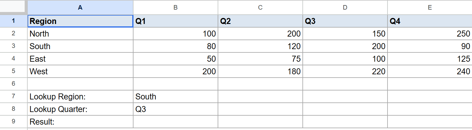
The goal is to look up the value at the intersection of the chosen region and chosen quarter, with both picked by name.

Here is the formula:

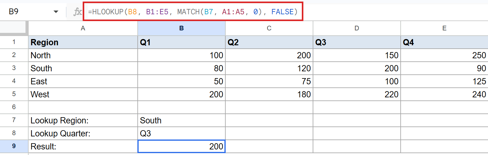
=HLOOKUP(B8, B1:E5, MATCH(B7, A1:A5, 0), FALSE)

Put it in B9.

How this formula works:

• MATCH(B7, A1:A5, 0) finds “South” inside the region column A1:A5. South sits in row 3 of that range (row 1 is the header “Region”, row 2 is North, row 3 is South). MATCH returns 3.
• That 3 becomes the third argument to HLOOKUP, which is the row index inside the lookup range.
• HLOOKUP("Q3", B1:E5, 3, FALSE) then looks for “Q3” in the first row of B1:E5, finds it in column D, and returns the value from row 3 of the range. Row 3 of B1:E5 is the South row, and the Q3 cell holds 200.

The formula returns 200, which matches South’s Q3 figure in the table. Change either input cell and the result updates automatically.

Pro Tip: This pattern works fine for small tables, but for new sheets consider XLOOKUP instead. XLOOKUP handles two-way lookups more directly and gives you cleaner error handling out of the box.

Tips & Common Mistakes

• The index is 1-based and counts rows inside the range, not the sheet. If your range starts at row 4 of the sheet, an index of 2 returns row 5, not row 2. People trip on this all the time, especially after inserting rows above the lookup table.
• The default is_sorted is TRUE, which is rarely what you want. Always pass FALSE explicitly for exact match. Leaving the argument off gives you approximate-match behavior, which silently returns the wrong value when the first row isn’t sorted. There’s no error, just bad data.
• HLOOKUP returns #N/A when no match is found. Wrap the formula in IFERROR for friendlier messaging: =IFERROR(HLOOKUP(A5, $A$1:$E$2, 2, FALSE), "Not found"). This is especially useful when the lookup is fed by user input that might not exist in the table.

Closing thought. HLOOKUP shows up far less often than VLOOKUP because people rarely lay data out horizontally.

But when the data is shaped that way, often in dashboards or quarter-by-quarter summaries, HLOOKUP is the cleanest way to pull values across a row.

For new sheets where you’re starting from scratch, XLOOKUP is the more modern choice, but HLOOKUP still has a place in any toolkit where you inherit a horizontal layout.

List of All Google Sheets Functions