If you want to pull a value from a specific position in a range, by row number, by column number, or both, the INDEX function in Google Sheets is what you’re looking for. You hand it a range and a position, and it returns whatever sits there.
In this article, I’ll walk you through five practical examples, from a plain position lookup to pairing INDEX with MATCH for a two-way lookup.
INDEX Function Syntax in Google Sheets
INDEX takes a range, then a row number, and optionally a column number.
=INDEX(reference, [row], [column])
reference: the range you want to pull a value from.row(optional): the row position inside the range. Row 1 is the first row of the range, not the sheet.column(optional): the column position inside the range. Needed when the range has more than one column.
If you set row or column to 0, INDEX returns the whole column or row instead of a single cell.
When to Use INDEX Function
- Grab a value by its position number when you already know the row or column.
- Build a two-way lookup by combining INDEX with MATCH.
- Return an entire column or row to feed into another function.
- Pull the last value in a list using a count as the position.
- Pick a cell from a grid using both a row and a column index.
Example 1: Return a value by its row position
Let’s start with the simplest case. You have a list of products and a column of position numbers, and you want the product that sits at each position.
Below is the dataset with product names in column A and the position you want in column B.
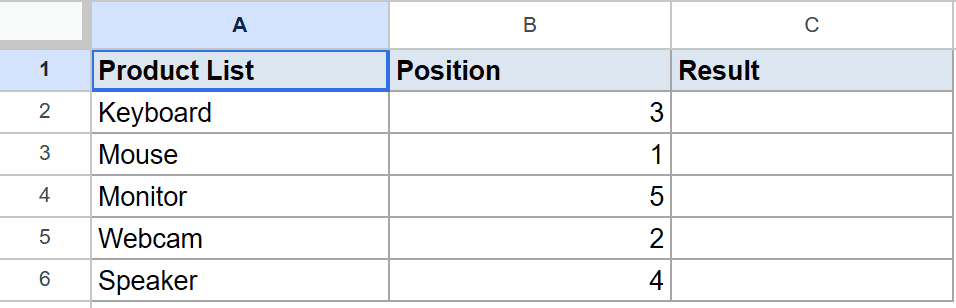
The goal is to return the product name that matches each position number.
Here is the formula:
=INDEX($A$2:$A$6,B2)
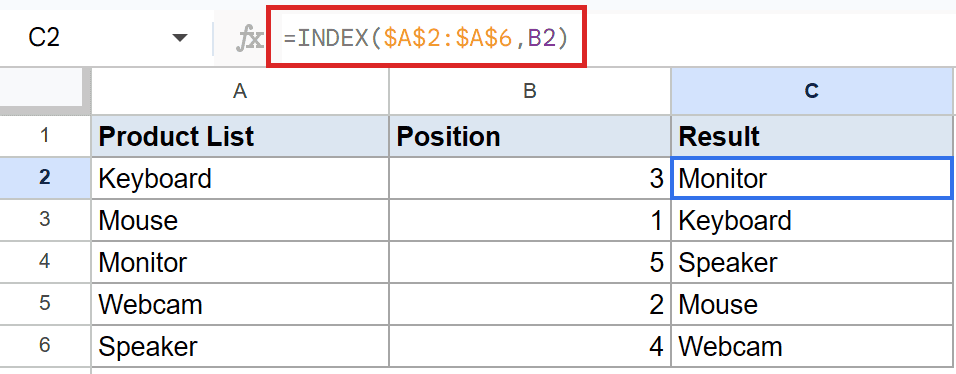
INDEX looks at the range A2:A6 and returns the item at the position in B2. B2 holds 3, so it returns Speaker, the third product in the list.
Filled down, B2’s position 3 gives Monitor, and the rest follow their own position numbers: Keyboard, Speaker, Mouse, and Webcam.
Pro Tip: If you’d rather use one formula instead of filling down, wrap INDEX in ARRAYFORMULA: =ARRAYFORMULA(INDEX($A$2:$A$6,B2:B6)). The result spills into the same cells.
Example 2: Pick a cell from a grid using row and column
INDEX can pull from a two-dimensional range when you give it both a row and a column number.
Below is the dataset with a small sales grid in A1:D5, plus a row index in column E and a column index in column F.
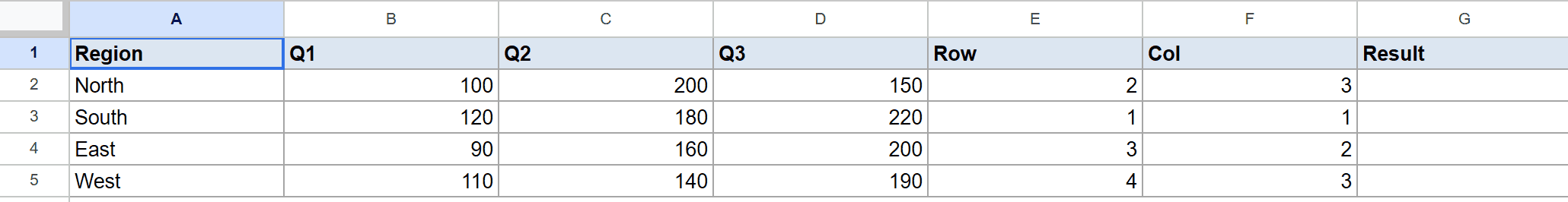
The goal is to return the value sitting at each row and column position inside the grid.
Here is the formula:
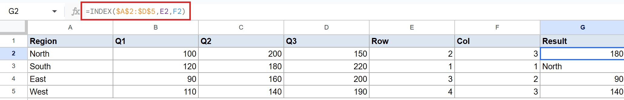
=INDEX($A$2:$D$5,E2,F2)
How this formula works:
- The range is A2:D5, so positions are counted from the top-left of that block.
- E2 is the row number and F2 is the column number.
- The first row asks for row 2, column 3, which returns 180.
- The next rows return North, then 90, then 140, each one a different cell from the grid.
Example 3: Two-way lookup with INDEX and MATCH
This is the pairing that makes INDEX so useful. On its own INDEX needs a position number, but you rarely know that number. MATCH finds it for you.
Below is the dataset with employee names in column A, IDs in column B, departments in column C, and a name to look up in column D.
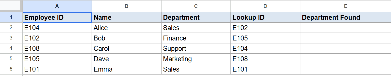
The goal is to return the department for each name in column D.
Here is the formula:
=INDEX($C$2:$C$6,MATCH(D2,$A$2:$A$6,0))
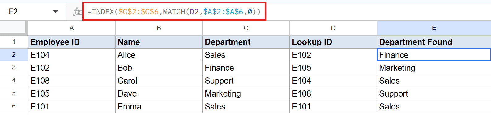
How this formula works:
- MATCH finds the position of the name in D2 inside the name list A2:A6.
- The
0tells the MATCH function to look for an exact match. - INDEX then returns the department at that same position from C2:C6.
- The first lookup returns
Finance, and the rest return Marketing, Sales, Support, and Sales.
Pro Tip: INDEX with MATCH works left or right, unlike VLOOKUP or the HLOOKUP function, which only search in a fixed direction. That makes this combo a flexible replacement for both.
Example 4: Return an entire column
Set the row argument to 0 and INDEX hands back the whole column instead of one cell.
Below is the dataset with order data in A1:C5, where column B holds the product names.
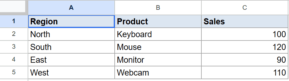
The goal is to return every value from the second column of the range in one shot.
Here is the formula:
=INDEX(A2:C5,0,2)
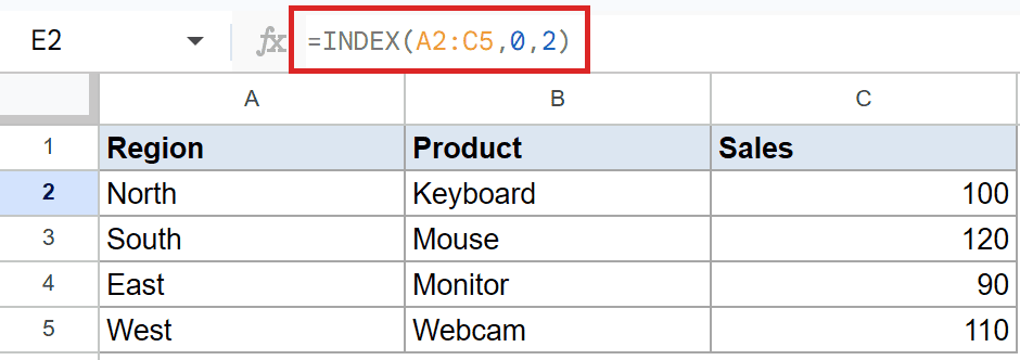
The 0 in the row spot tells INDEX to skip picking a single row and return the full column. The 2 points at the second column, the product names.
The result spills down the cells below the formula: Keyboard, Mouse, Monitor, and Webcam. Only the top cell holds a formula. The rest fill in automatically.
Example 5: Get the last value in a list
INDEX paired with COUNTA is a clean way to grab the last entry in a column, even as the list grows.
Below is the dataset with months in column A and sales figures in column B.
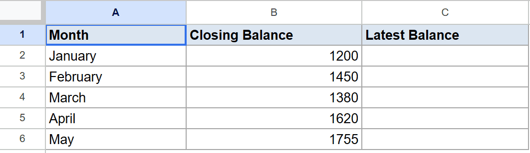
The goal is to return the most recent sales value, the last one in the column.
Here is the formula:
=INDEX(B2:B6,COUNTA(B2:B6))
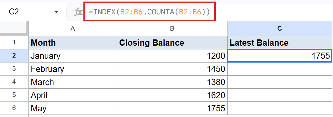
COUNTA counts how many values are in B2:B6, which is 5. INDEX then returns the value at position 5, the last one in the range.
The result is 1755. If you add more months, COUNTA grows with them, so the formula always points at the latest figure.
Tips & Common Mistakes
- Positions count from the range, not the sheet. Row 1 in INDEX means the first row of your reference, not row 1 of the spreadsheet. Forgetting this is the most common slip.
- Lock your range with absolute references when filling down. Without the dollar signs, the range shifts as you copy the formula. Examples 1 and 3 use
$A$2:$A$6so the range stays put. - Pair INDEX with MATCH for real lookups. A hard-coded position number breaks the moment your data moves. Let the MATCH function find the position so the formula keeps working.
INDEX looks plain at first, since all it does is return a value by position. The moment you pair it with MATCH or set an argument to 0, it turns into a flexible lookup and range tool that handles jobs VLOOKUP can’t.
List of All Google Sheets Functions
Related Google Sheets Functions / Articles: