If you need a random whole number between two bounds, the RANDBETWEEN function in Google Sheets gives you one in a single call.
It takes a low value and a high value, and returns a random integer somewhere in that range, both ends included. In this article, I’ll show you how to use RANDBETWEEN with a few practical examples.
RANDBETWEEN Function Syntax in Google Sheets
Here is how the RANDBETWEEN function is written:
=RANDBETWEEN(low, high)
- low is the smallest integer you want to allow. Can be a number, a cell reference, or any expression that resolves to a number.
- high is the largest integer you want to allow. Same rules as low.
Both ends are inclusive, so =RANDBETWEEN(1,6) can return 1, 6, or anything in between.
One thing to know up front: RANDBETWEEN is a volatile function. The value changes on every recalculation, which is what makes it useful for simulations but a pain when you wanted a fixed result.
When to Use RANDBETWEEN Function
- Generate random test data for a column when you don’t have real numbers yet.
- Simulate dice rolls, coin flips, or any other discrete random event.
- Assign random IDs, sample numbers, or seat positions in a quick spreadsheet.
- Pair with INDEX or CHOOSE to pick a random item from a list.
- Generate a random calendar date inside a window by feeding DATE values as the bounds.
Example 1: Random Integer Between 1 and 100
Let’s start with the simplest use, generating a random number between two fixed bounds.
Below is the dataset, with a Trial label in A1 and the numbers 1 through 6 in column A as row markers.
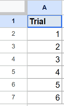
You want each row in column B to show a random integer between 1 and 100.
Here is the formula:
=RANDBETWEEN(1,100)
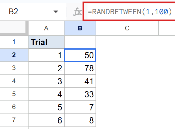
RANDBETWEEN picks a random integer in the inclusive range you pass it. Every cell that holds this formula gets its own draw, so each trial row shows a different number between 1 and 100.
If you edit any cell in the sheet, every RANDBETWEEN formula recalculates and the numbers shuffle. That’s normal behavior, not a bug.
Pro Tip: RANDBETWEEN only returns whole numbers. If you need a random decimal, divide the result by a factor, like `=RANDBETWEEN(1,1000)/100` for a number with two decimal places. For an unbounded decimal between 0 and 1, use RAND instead.
Example 2: Simulate Dice Rolls for a Player List
A common use of RANDBETWEEN is simulating a die. Just set the low to 1 and the high to the number of faces.
Below is the dataset, with a Player label in A1 and six player names in column A, rows 2 to 7.
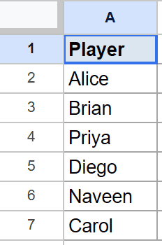
You want each player in column B to show a random dice roll between 1 and 6.
Here is the formula:
=RANDBETWEEN(1,6)
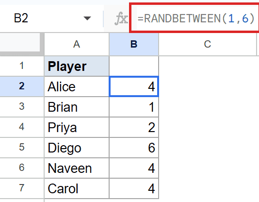
Same shape as Example 1, just with a tighter range. Each cell in column B gets its own roll between 1 and 6, inclusive.
Want a twenty-sided die? Change 6 to 20. The formula doesn’t care what the upper bound is, as long as it’s an integer larger than the low.
Example 3: Use Cell References for Low and High
The bounds don’t have to be hardcoded numbers. Passing them as cell references lets you tweak the range without editing every formula.
Below is the dataset, with Low, High, and Random as headers in row 1. Column A holds the low value, column B holds the high value, and column C is where the random number will land.
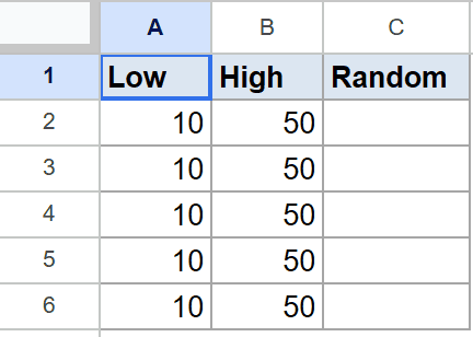
You want each row in column C to pick a random integer based on the low and high in that same row.
Here is the formula:
=RANDBETWEEN(A2,B2)
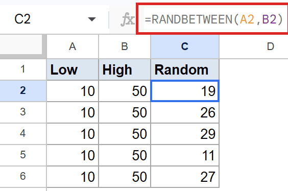
Each row reads its own low and high from columns A and B, so you can change either bound and the random number for that row stays inside the new range.
This pattern is useful when different rows need different ranges, or when you want to control the bounds from a couple of input cells at the top of the sheet.
Example 4: Pick a Random Name From a List
RANDBETWEEN really shines when you nest it inside INDEX. The random number becomes a row position, and INDEX hands back whatever sits at that row.
Below is the dataset, with an Employee label in A1 and six names in column A, rows 2 to 7.
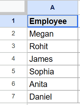
You want cell C2 to show a random name from the list, regardless of which row it lives on.
Here is the formula:
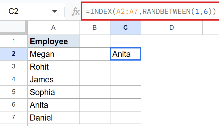
=INDEX(A2:A7,RANDBETWEEN(1,6))
How this formula works:
- RANDBETWEEN(1,6) picks a random integer between 1 and 6.
- INDEX takes the range A2:A7 and the random integer, then returns the name in that row of the range.
- Every recalculation picks a new row, so the displayed name shuffles.
This is the classic random-picker pattern. Use it for raffle draws, random sampling, or any time you need one item from a list without thinking about it.
Pro Tip: Match the upper bound to the row count of your list. If the list grows to seven names, change the formula to `=INDEX(A2:A8,RANDBETWEEN(1,7))`. Or make it dynamic with `=INDEX(A2:A8,RANDBETWEEN(1,COUNTA(A2:A8)))` so the formula keeps working when you add or remove rows.
Example 5: Generate a Random Date in a Year
Dates in Google Sheets are stored as serial numbers under the hood, which means RANDBETWEEN can pick a random date the same way it picks a random number. Wrap each end in a DATE call and you’re done.
Below is the dataset, with a Trial label in A1 and trial numbers 1 through 6 in column A.

You want each row in column B to show a random date somewhere in the year 2026.
Here is the formula:
=RANDBETWEEN(DATE(2026,1,1),DATE(2026,12,31))
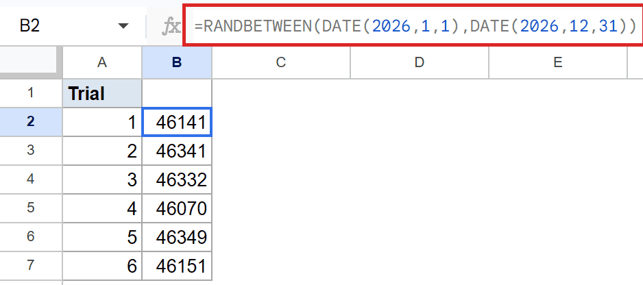
DATE(2026,1,1) and DATE(2026,12,31) hand RANDBETWEEN two integers under the hood. It picks a random whole number between them, which happens to land on a date inside 2026.
The result cell will show the number unless you format it as a date. Select the column, then Format menu, Number, Date, and the serial flips into a readable date.
Tips & Common Mistakes
- RANDBETWEEN is volatile. The value changes every time the sheet recalculates, which happens whenever you edit any cell, refresh, or reopen the file. To freeze a value once you like it, copy the cell, then Edit menu, Paste special, Values only. The number stops changing.
- Both bounds must be integers. Pass a decimal and Google Sheets truncates it to an integer before evaluating.
=RANDBETWEEN(1.5,10)works as if you wrote=RANDBETWEEN(1,10). If you need a random decimal, use RAND directly or divide a RANDBETWEEN result by a scale factor. - The low must be less than or equal to the high. Swap them and Google Sheets returns a
#NUM!error. If your bounds come from cell references and you’re not sure which is bigger, wrap them in MIN and MAX, like=RANDBETWEEN(MIN(A1,B1),MAX(A1,B1)).
RANDBETWEEN is a small function that earns its keep across simulations, test data, and random-picker tricks. Set the bounds, drop it into a cell, and you have a random integer.
Pair it with INDEX when you need a random list item, with DATE when you want a random calendar day, or with paste-special-values when you want a single draw that stays put.