
If you want to pull characters from the start of a text string, the LEFT function in Google Sheets gives you the first N characters in one step. In this article I’ll show you five examples covering fixed-length prefixes, name initials, delimiter-based splits, per-row character counts, and prefix matching with IF.
LEFT Function Syntax in Google Sheets
Here is what the function looks like.
=LEFT(string, [number_of_characters])
- string – the text you want to pull characters from (a string in quotes, or a cell reference).
- number_of_characters – how many characters to return from the left side, [optional]. Defaults to 1 if you leave it blank.
When to Use LEFT Function
- Extract a fixed prefix from a code or ID column.
- Pull the first letter of a name to build initials.
- Combine with FIND to split a string at a delimiter like a space or dash.
- Drive the character count from another cell so each row gets a different slice.
- Test a prefix inside IF to label or flag rows based on how they start.
Example 1: Extract the First Three Characters
Let’s start with the simplest case, where every row gets the same number of characters from the left.
Below is the dataset, with product codes in column A. Each code starts with a country prefix followed by some other parts joined by dashes.
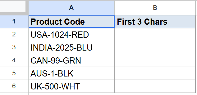
I want each row to return just the first 3 characters of the code.
Here is the formula:
=LEFT(A2,3)
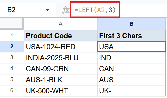
LEFT just walks 3 characters in from the start and returns whatever it grabbed. Notice the last row: “UK-500-WHT” is only 2 letters before the first dash, so LEFT returns “UK-” (including the dash). LEFT counts every character, dashes and spaces included.
Pro Tip: To run this across a whole column at once, wrap the call in ARRAYFORMULA like this: =ARRAYFORMULA(LEFT(A2:A6, 3)). No need to fill down.
Example 2: Grab the First Initial of a Name
The number-of-characters argument can be any positive integer, including 1.
Below is the dataset, with first names in column A.
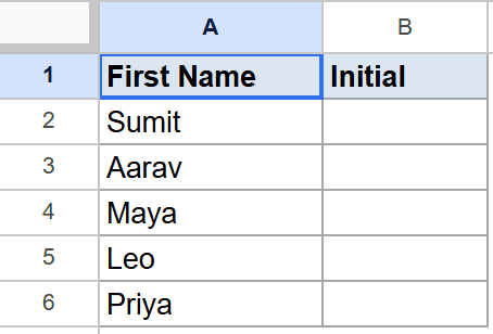
I want each row to return just the first letter of the name.
Here is the formula:
=LEFT(A2,1)
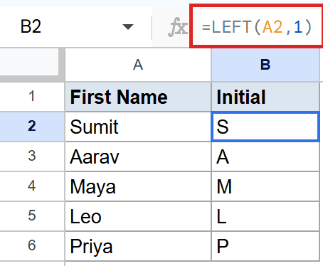
Passing 1 as the second argument gives you the very first character. Useful when you’re building initials or short codes from a name list.
Example 3: Pull the First Name From a Full Name
When the number of characters isn’t fixed, you can compute it from the string itself.
Below is the dataset, with full names in column A. Each name has the first and last separated by a space.
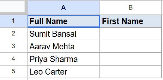
I want each row to return just the first name, before the space.
Here is the formula:
=LEFT(A2,FIND(" ",A2)-1)
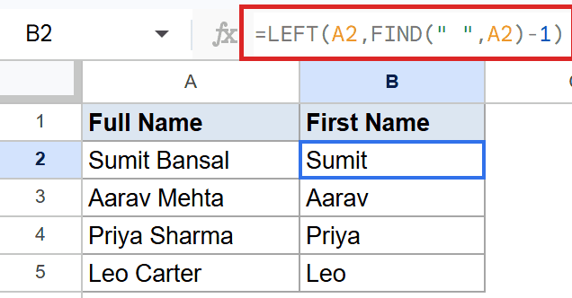
How this formula works:
- FIND(” “, A2) returns the position of the first space. For “Sumit Bansal” that’s 6.
- Subtracting 1 gives you the count of characters before the space (5 in this case).
- LEFT then pulls that many characters from the start, returning “Sumit”.
Pro Tip: If your text doesn’t always contain a space (some rows might be just a single name), wrap FIND in IFERROR so the formula returns the whole string instead of a #VALUE! error. SPLIT is also worth a look for delimiter-based extraction when you want all parts at once.
Example 4: Variable Length Per Row
You can drive the character count from a second column, so each row gets a different slice.
Below is the dataset, with text strings in column A and the desired length in column B.
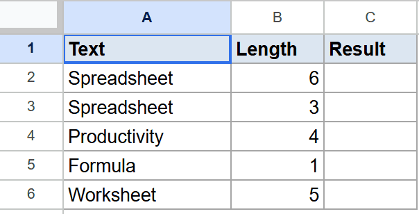
I want column C to show the LEFT result, using the per-row count from column B.
Here is the formula:
=LEFT(A2,B2)
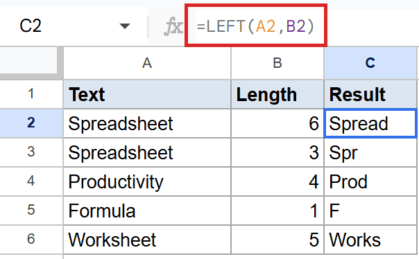
LEFT simply uses whatever number sits in column B. So “Spreadsheet” with 6 gives “Spread”, “Productivity” with 4 gives “Prod”, and “Formula” with 1 gives “F”.
Example 5: Flag Rows by Their Prefix
LEFT is often dropped inside an IF to label rows by what they start with.
Below is the dataset, with codes in column A. Each code starts with a 2-letter country prefix.
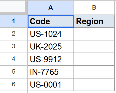
I want column B to say “US Code” for rows that start with “US” and “Other” for the rest.
Here is the formula:
=IF(LEFT(A2,2)="US","US Code","Other")
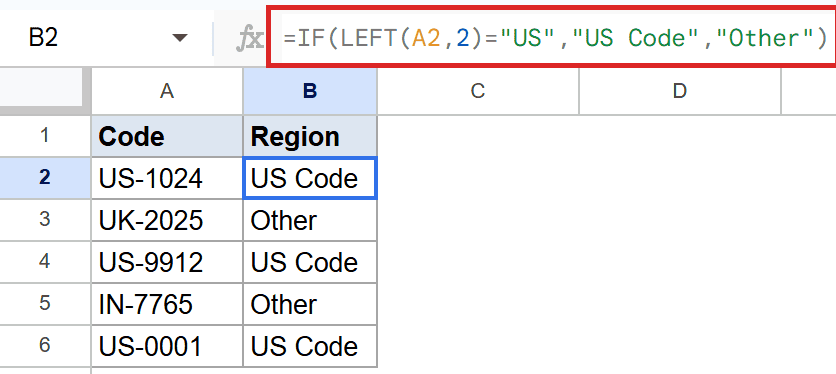
LEFT extracts the first 2 characters of each code, then IF compares it against “US”. When it matches, the cell shows “US Code”; otherwise it shows “Other”. Notice how rows starting with “UK” and “IN” both fall into the “Other” bucket.
Tips & Common Mistakes
- LEFT counts every character. Dashes, spaces, and punctuation all count. If you only want letters, strip the extras first with SUBSTITUTE before passing to LEFT.
- N larger than the string is fine. If you ask for 10 characters from a 5-character string, LEFT just returns the whole 5-character string without erroring out. Pair with LEN if you need to check length first.
- LEFT only walks from the start. For characters from the end of the string, use RIGHT. For a slice from the middle, use MID. Same family, different starting point.
That covers the main ways to use LEFT in Google Sheets. The function is most useful when you pair it with FIND for delimiter splits, with LEN for length-aware extractions, or inside IF to drive labels off the first few characters of a code.
List of All Google Sheets Functions
Related Google Sheets Functions / Articles: