
When you need to check whether a cell holds an actual number rather than text, a blank, or an error, the ISNUMBER function in Google Sheets gives you a clean TRUE or FALSE. This article shows five examples that cover the common checks and combos you’ll reach for.
ISNUMBER Function Syntax in Google Sheets
The function takes a single value or cell reference.
=ISNUMBER(value)
- value – the cell, value, or expression you want to test; ISNUMBER comes back TRUE if it evaluates to a number
When to Use ISNUMBER Function
- Spotting numbers stored as text after a paste or import
- Filtering a mixed column so calculations skip non-numeric rows
- Pairing with SEARCH or FIND to check if a string contains a substring
- Counting how many numeric values sit inside a range
- Building safer formulas that don’t break on text or blank cells
Example 1: Test a mixed column for numeric values
Let’s start with the simplest case, a single column with a mix of numbers, text, and a blank.
Below is the dataset, with values 42, 3.14, the word hello, an empty cell, and -7 in cells A2 to A6.
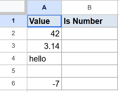
The goal is to put TRUE next to each numeric value and FALSE next to anything that isn’t a number.
Here is the formula:
=ISNUMBER(A2)
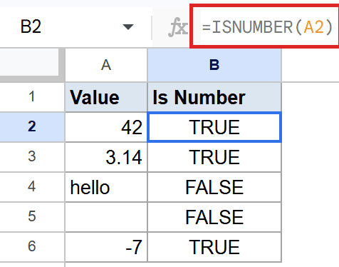
ISNUMBER checks the value in A2 and comes back TRUE for the first two rows, FALSE for “hello” and the blank cell, then TRUE again for -7. Drag the formula down to fill the rest of column B.
Pro Tip: ISBLANK and ISTEXT are the sibling checks for empty cells and text strings. Wrap ISNUMBER inside IFERROR if you want to catch error values without converting them to text.
Example 2: Spot numbers stored as text
Imports from CSVs or pasted data often leave numbers stored as text, and ISNUMBER catches them.
Below is the dataset, with the entries 100, “100 USD”, 50, “fifty”, and “2024” sitting in cells A2 to A6. Some look numeric but are actually text.
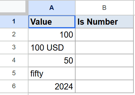
You want to flag the cells that are real numbers and the ones that only look like numbers.
Here is the formula:
=ISNUMBER(A2)
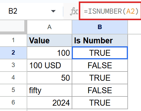
ISNUMBER comes back TRUE for the rows with 100, 50, and “2024” stored as a number. It comes back FALSE for “100 USD” (text because of the unit) and “fifty” (a spelled-out word).
This is a quick way to audit a column before running totals or averages.
Example 3: Skip non-numbers in a calculation
ISNUMBER is most useful inside the IF function, where it acts as a safety gate for math operations.
Below is the dataset, with values 10, “abc”, 25, a blank, and 7.5 in cells A2 to A6. You want to double the numbers and label everything else.
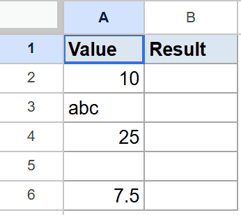
The goal is to multiply each numeric cell by 2 and put the word Skip in rows that contain text or are empty.
Here is the formula:
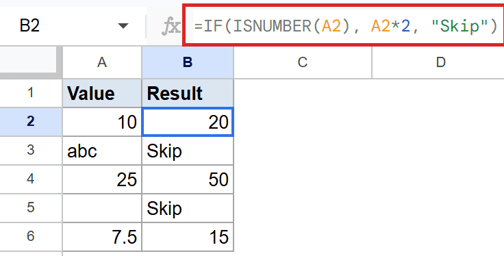
=IF(ISNUMBER(A2), A2*2, "Skip")
How this formula works:
- ISNUMBER(A2) is the test that returns TRUE or FALSE.
- If TRUE, IF returns A2*2, so 10 becomes 20, 25 becomes 50, and 7.5 becomes 15.
- If FALSE, IF returns the text “Skip” instead, keeping the column clean.
Example 4: Check if a string contains an @ symbol
A classic ISNUMBER combo is pairing it with SEARCH to test whether a substring exists inside a longer string.
Below is the dataset, a list of values in A2 to A6 that includes valid email addresses like alice@example.com and non-emails like “bob_at_test” and “dan”.
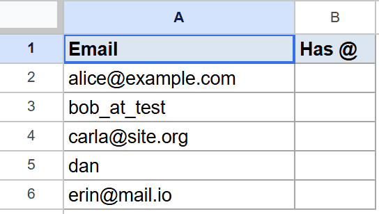
The goal is to flag any value that contains the @ character as a basic email-check.
Here is the formula:
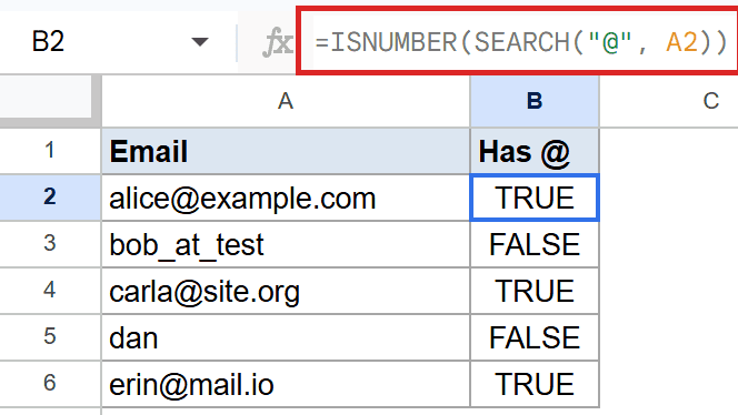
=ISNUMBER(SEARCH("@", A2))
How this formula works:
- SEARCH looks for the @ symbol inside the cell value.
- When @ is found, SEARCH returns the position number, which is a number.
- When @ is missing, SEARCH returns a #VALUE! error.
- ISNUMBER converts the position into TRUE and the error into FALSE, giving you a clean flag column.
Example 5: Count how many numbers are in a range
Pair ISNUMBER with SUMPRODUCT and you get a quick count of all numeric cells inside a mixed range.
Below is the dataset, with 10, “text”, 25, a blank, and 7.5 in cells A2 to A6.
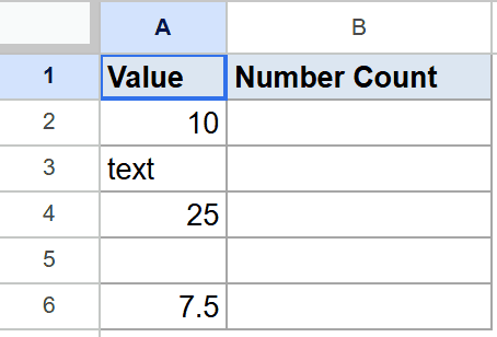
You want to count how many cells in that range actually hold a number, all in a single formula.
Here is the formula:
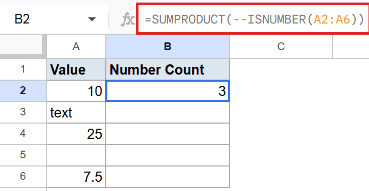
=SUMPRODUCT(--ISNUMBER(A2:A6))
How this formula works:
- ISNUMBER(A2:A6) returns an array of TRUE/FALSE for each cell.
- The double-negative (
--) converts TRUE to 1 and FALSE to 0. - SUMPRODUCT adds the 1s and 0s, so the formula returns 3 because three cells (10, 25, 7.5) are numbers.
Tips & Common Mistakes
- ISNUMBER ignores formatting. A cell can display “$100” but ISNUMBER still returns TRUE because the underlying value is a number. Format does not change the type.
- Pair with SUMIF function for safer sums. If a column has mixed types, ISNUMBER-based array logic protects your totals from text-induced errors.
- TRUE/FALSE are not 1/0. ISNUMBER’s output is boolean. To use it in arithmetic, coerce with double-negative or multiply by 1.
ISNUMBER is the type-checker you’ll reach for any time a column might hold mixed content. It’s most useful inside larger formulas with IF, SEARCH, or SUMPRODUCT, where the boolean result acts as a switch. Three or four small uses save a lot of cleanup later.
List of All Google Sheets Functions
Related Google Sheets Functions / Articles: