BYROW Function in Google Sheets

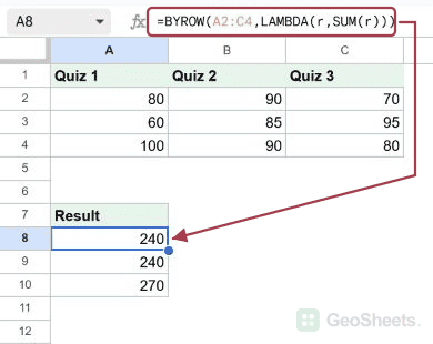
If you want to run a calculation across each row of a range and get one result per row, the BYROW function in Google Sheets is what you reach for. It pairs with a LAMBDA so you can plug in any per-row logic you like.

In this article, I’ll show you how to use BYROW with five practical examples covering sums, maximums, averages, conditional counts, and text joins.

BYROW Function Syntax in Google Sheets

Here is how you write the BYROW function.

=BYROW(array_or_range, LAMBDA(row, expression))
  • arrayorrange – the 2D range you want to process one row at a time.
  • LAMBDA(row, expression) – a LAMBDA where row is the placeholder for each row and expression is the calculation you run on it.

The result spills down one cell per input row.

When to Use BYROW Function

  • When you need a per-row total, max, min, average, or count from a 2D range.
  • When you want one formula that handles every row instead of filling a formula down.
  • When the per-row logic needs more than a basic operator, like a COUNTIF or TEXTJOIN.
  • When you want a single spilling result that grows automatically with the input range.

Example 1: Sum each row of a numeric range

Let’s start with the most common use, summing each row.

Below is the dataset, three columns of quarterly numbers in A2 to C6.

Google Sheet showing example dataset with Q1, Q2, Q3 headers and numeric values.

The goal is to get the row total for each row in a single spilling formula.

Here is the formula:

=BYROW(A2:C6, LAMBDA(r, SUM(r)))
Google Sheets displaying a BYROW LAMBDA formula in D2 summing rows A2:C6.

BYROW walks A2:C6 one row at a time. For each row it hands the row to the LAMBDA, which sums it. The five totals spill down from D2 to D6.

Pro Tip: To do the same calculation column by column instead of row by row, swap BYROW for BYCOL. Same syntax, different axis.

Example 2: Find the max value in each row

Same shape, different aggregator.

Below is the dataset, monthly sales for five products in A2 to C6.

Google Sheets: Jan, Feb, Mar headers above five rows of numerical data.

The goal is to find the highest month for each product.

Here is the formula:

=BYROW(A2:C6, LAMBDA(r, MAX(r)))
`=BYROW(A2:C6, LAMBDA(r, MAX(r)))` formula in D2 calculates the max value per row.

The LAMBDA runs MAX on each row, and BYROW spills five values down. Product 1 peaks at 78, product 2 at 89, and so on.

Example 3: Average each student’s test scores

You can plug AVERAGE into the LAMBDA the same way.

Below is the dataset, a name in column A and three test scores in B2 to D6.

Google Sheets dataset: Student names and scores for Test1, Test2, and Test3.

The goal is to compute each student’s mean across the three tests.

Here is the formula:

=BYROW(B2:D6, LAMBDA(r, AVERAGE(r)))
Google Sheets BYROW formula in E2 averages student test scores from B2:D6.

BYROW only walks B2:D6, the score columns, so the name column stays untouched. Emma averages 84.33, Liam 80.33, and the rest follow.

Example 4: Count high scores per row with COUNTIF

The LAMBDA body can be any expression that returns a single value, including a COUNTIF.

Below is the dataset, three quiz scores per student in B2 to D6.

Google Sheet: student names and scores for Quiz1, Quiz2, Quiz3.

The goal is to count how many quizzes each student scored 80 or above.

Here is the formula:

=BYROW(B2:D6, LAMBDA(r, COUNTIF(r, ">=80")))
Google Sheet showing BYROW formula in E2 counting quiz scores >=80 per row.

For each row, COUNTIF tallies how many cells meet >=80. Sophia gets all three, Lucas gets one, and the rest land in between.

Pro Tip: If you’d rather use a fill-down formula instead of BYROW, you can wrap COUNTIF in ARRAYFORMULA, though the LAMBDA version is cleaner when the per-row logic gets more complex.

Example 5: Concatenate first and last names per row

BYROW works with text too.

Below is the dataset, first names in column A and last names in column B.

Sheets table with 'First' and 'Last' name columns and four rows of example data.

The goal is to merge each row into a single full name.

Here is the formula:

=BYROW(A2:B5, LAMBDA(r, TEXTJOIN(" ", TRUE, r)))
BYROW formula in C2 spills combined names from A2:B5, starting with John Smith.

TEXTJOIN stitches the two cells of each row together with a space. The result spills four full names from C2 down.

Tips & Common Mistakes

  • Match the LAMBDA argument to the row variable – the placeholder name inside LAMBDA is up to you (r, row, x), but you must reference the same name inside the expression. A typo there gives a #NAME error.
  • BYROW expects a single value per row – the LAMBDA body must return one value. If you write a formula that returns an array per row, you’ll get a #VALUE error. Use MAP instead for that case.
  • Use BYCOL for the column version – BYROW collapses each row into a single value. If you want to collapse each column instead, swap in BYCOL with the same syntax.

BYROW is the cleanest way to run any per-row aggregator across a 2D range. Once you’re comfortable with LAMBDA syntax, you can drop in SUM, MAX, AVERAGE, COUNTIF, TEXTJOIN, or anything else that returns one value.

That covers BYROW with five solid examples. Pair it with BYCOL for column-wise work and you’ve got both axes handled.

List of All Google Sheets Functions

Related Google Sheets Functions / Articles: