
If you want to count the number of working days between two dates, the NETWORKDAYS function in Google Sheets does it in one shot. It counts Monday through Friday and skips weekends automatically.
In this article, I’ll walk you through NETWORKDAYS with five examples, from a simple two-date count to excluding holidays and comparing calendar days against workdays.
NETWORKDAYS Function Syntax in Google Sheets
Here is how you write the NETWORKDAYS function.
=NETWORKDAYS(start_date, end_date, [holidays])
- start_date – the beginning date of the range.
- end_date – the ending date of the range.
- holidays – optional. A range of dates or an array literal of dates to exclude on top of weekends.
The function is inclusive of both the start and end date if they fall on weekdays. It returns an integer.
When to Use NETWORKDAYS Function
- Counting billable workdays for invoicing.
- Calculating project duration in working days, not calendar days.
- Figuring out how many business days are left until a deadline.
- Excluding weekends and company holidays from any date-range total.
Example 1: Basic workdays between two dates
Let’s start with the simplest case, two hardcoded dates and no holidays.
Below is the dataset, a description in column A and an empty Working Days cell in B2.

The goal is to count the workdays from January 5, 2026 to January 30, 2026.
Here is the formula:
=NETWORKDAYS("2026-01-05", "2026-01-30")
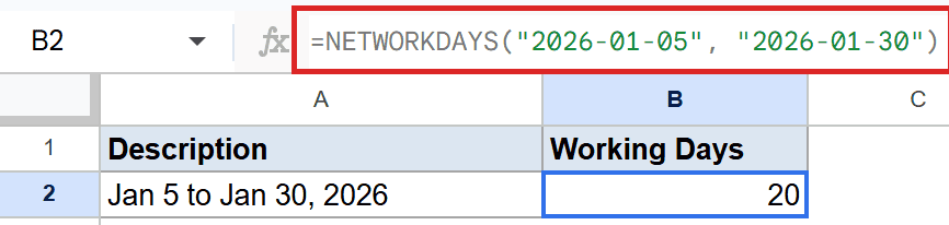
The function counts every Monday through Friday between the two dates, both ends included. The result lands at 20 working days.
Example 2: Workdays per row from cell references
In most real datasets your dates live in cells, not in the formula itself.
Below is the dataset, a start date in column A and an end date in column B for five date pairs.
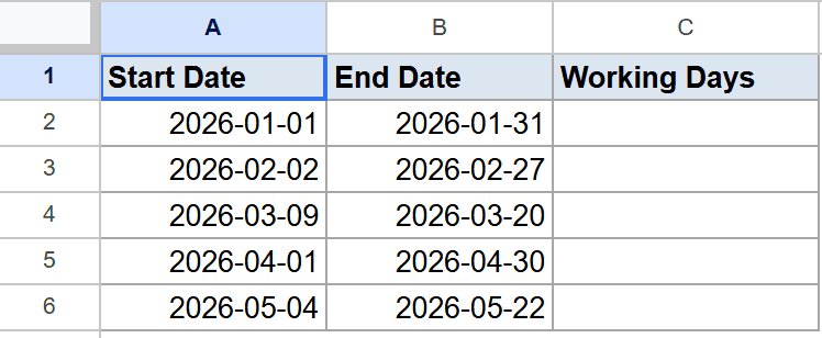
The goal is to get the working days for each row in column C.
Here is the formula:
=NETWORKDAYS(A2, B2)
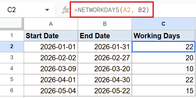
Drop this in C2 and fill it down. Each row counts the workdays between its own start and end date. January gives 22, February 20, and the rest follow.
Example 3: Exclude holidays with an array literal
The third argument lets you exclude specific holiday dates on top of the weekend skip.
Below is the dataset, a single date range that brackets Christmas week.

The goal is to count workdays from December 22 to December 31, 2026, while skipping December 25 and 26.
Here is the formula:
=NETWORKDAYS("2026-12-22", "2026-12-31", {DATE(2026,12,25); DATE(2026,12,26)})

The curly braces with semicolons build an inline array of holiday dates, no separate range needed. The result is 7 workdays. Sheets pulls out weekends plus the two holidays.
Pro Tip: The array literal uses semicolons as row separators in Google Sheets. If you prefer, you can list the holidays in a column and pass that range as the third argument instead.
Example 4: Project workdays excluding a holiday range
You can pass a range of holiday cells as the third argument too, which is cleaner for company calendars.
Below is the dataset, project start and end in columns A and B, and three company holidays sitting in C2 to C4.

The goal is to count working days from July 1 to July 31, 2026, excluding the three holidays.
Here is the formula:
=NETWORKDAYS(A2, B2, C2:C4)
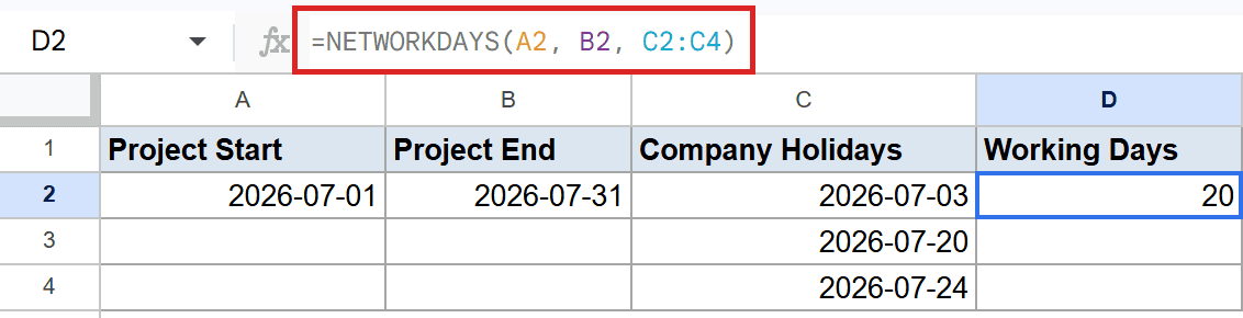
NETWORKDAYS reads the holiday range, removes any of those dates from the count, and returns 20 working days for July.
Example 5: Compare calendar days vs working days
You can pair NETWORKDAYS with DAYS to figure out how many non-working days fall inside a range.
Below is the dataset, a single description row.

The goal is to count the non-working days between January 1 and April 30, 2026.
Here is the formula:
=DAYS("2026-04-30", "2026-01-01") - NETWORKDAYS("2026-01-01", "2026-04-30")

DAYS gives the total calendar gap. Subtracting NETWORKDAYS leaves just the weekends. The result is 33 non-working days.
Tips & Common Mistakes
- Both endpoints are inclusive – if your start and end dates are both weekdays, NETWORKDAYS counts both of them. Mon to Fri is 5, not 4.
- Use NETWORKDAYS.INTL for non-standard weekends – NETWORKDAYS hard-codes Saturday and Sunday as the weekend. If your weekend is Friday-Saturday or just Sunday, switch to NETWORKDAYS.INTL where you control which days count as weekends.
- Invalid date strings return #VALUE – pass dates as real date values, cell references, or ISO strings like
"2026-01-30". A typo like"Jan 30th"will trip the function.
NETWORKDAYS handles the most common date math you’ll need at work, business days between two points, with optional holiday handling baked in. Combine it with DAYS for non-working-day counts and with NETWORKDAYS.INTL when your weekend doesn’t sit on Saturday and Sunday.
List of All Google Sheets Functions
Related Google Sheets Functions / Articles: