COLUMN Function in Google Sheets

If you want to get the column number of a cell or build a list of sequential numbers across a row, the COLUMN function in Google Sheets is the function you want.

It returns the column number of any reference you pass in, or the formula’s own column if you call it with no argument. In this article,

I’ll walk you through four practical examples that cover reading a column number from a text reference, returning the current column, spilling a sequence across a row, and converting a column number back into a letter.

COLUMN Function Syntax in Google Sheets

COLUMN takes at most one argument.

=COLUMN([cell_reference])

• cell_reference (optional): the cell or range whose column number you want. If you omit it, COLUMN returns the column number of the cell that contains the formula.

When you pass a single cell, COLUMN returns a single number. When you pass a range, it returns the column numbers across that range (use ARRAYFORMULA so the result spills).

When to Use COLUMN Function

• Build a dynamic column index for use inside INDEX, OFFSET, or VLOOKUP.
• Generate a row of sequential numbers (1, 2, 3, …) for headers, IDs, or progress trackers.
• Detect which column the current formula is in so the same formula behaves differently in different columns.
• Convert a cell reference written as text into its column number by combining COLUMN with INDIRECT.
• Pair with ADDRESS to flip a column number back into a letter for labels or audit notes.

Example 1: Get the column number from a cell reference

Let’s start with the most direct use. You have a cell reference written as text, and you want the column number for it.

Below is a small table with five cell references typed in column A.

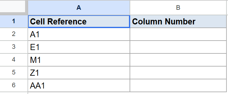
The goal is to return the column number for each reference in column B.

Here is the formula:

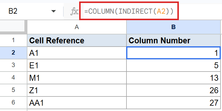
=COLUMN(INDIRECT(A2))

Put it in B2 and fill it down through B6.

How this formula works:

• INDIRECT takes the text in A2 (“A1”) and turns it into a live cell reference.
• COLUMN reads that reference and returns its column number.
• A1 is column 1, E1 is column 5, M1 is column 13, Z1 is column 26, and AA1 is column 27 (the column right after Z).

Pro Tip: ROW is the row equivalent of COLUMN. If you ever need the row number from a text reference, swap COLUMN for ROW: =ROW(INDIRECT(A2)) returns the row number instead.

Example 2: Get the column number of the current cell

Call COLUMN with no argument and it returns the column number of the cell holding the formula itself. Useful when you want a formula to behave differently depending on which column it’s in.

Below is a small note showing where the formula sits.

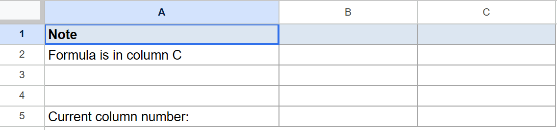
The goal is to confirm that COLUMN with no argument returns the column number of the formula cell.

Here is the formula:

=COLUMN()

Put it in C5.

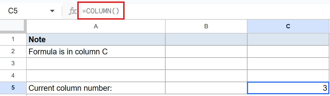
C5 returns 3, because the formula sits in column C and column C is the third column. Move the same formula to column F and it would return 6.

This is the part that surprises people the first time they see it. COLUMN with no argument does not return the column of any data, it returns the column of the cell containing the formula.

Pro Tip: This is the trick that makes formulas portable. Combine COLUMN() with subtraction (e.g. COLUMN()-1) to generate a sequential index that updates automatically as you drag the formula across columns.

Example 3: Generate a sequence of column numbers in one shot

Pass a horizontal range to COLUMN and it returns the column number for every cell in that range. Wrap the call in ARRAYFORMULA and the result spills across the row.

Below is an empty header row with five “Col” labels.

The goal is to fill A2 through E2 with the numbers 1, 2, 3, 4, 5 using a single formula.

Here is the formula:

=ARRAYFORMULA(COLUMN(A1:E1))

Put it in A2.

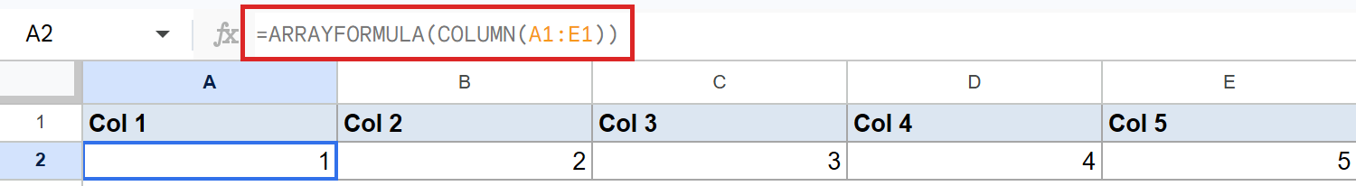
COLUMN reads every cell in the A1:E1 range and returns the column number for each one.

ARRAYFORMULA tells Google Sheets to spill the result across A2:E2 instead of collapsing it to a single value. You get 1, 2, 3, 4, 5 without typing any number.

Pro Tip: This is a quick way to generate a numeric header row that auto-adjusts if you change the input range. SEQUENCE does the same thing more explicitly (=SEQUENCE(1,5) produces the same row), but the COLUMN + ARRAYFORMULA pattern shows up often in older sheets and inside larger array formulas.

Example 4: Convert a column number back into a column letter

COLUMN gives you a column number. Sometimes you need to flip back the other way and get the column letter from a number.

The cleanest way is to combine the ADDRESS function with SUBSTITUTE.

Below is a table of column numbers in column A.

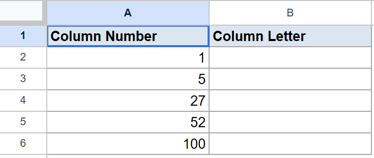
The goal is to return the matching column letter for each number in column B.

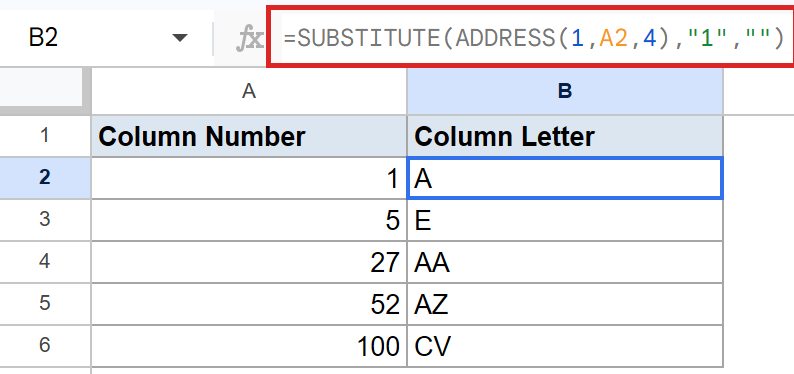
Here is the formula:

=SUBSTITUTE(ADDRESS(1,A2,4),"1","")

Put it in B2 and fill it down through B6.

How this formula works:

• ADDRESS(1, A2, 4) builds a relative cell reference for row 1 and column number A2. With mode 4 (fully relative), the result is something like A1, E1, AA1, AZ1, or CV1 (no dollar signs).
• SUBSTITUTE(..., "1", "") strips the 1 off the end, leaving just the column letter.
• Column 1 returns A, column 5 returns E, column 27 returns AA, column 52 returns AZ, and column 100 returns CV.

Pro Tip: COLUMN returns a number, ADDRESS returns text, so the two are complementary. COLUMN gets you the number from a reference, and ADDRESS + SUBSTITUTE gets you the letter from a number. Together they’re the standard pair for column conversions in Google Sheets.

Tips & Common Mistakes

• COLUMN with no argument refers to the formula cell, not a fixed column. This is the most common surprise. =COLUMN() placed in C5 returns 3, but the same formula in F5 returns 6. If you want a fixed column number that doesn’t change, pass an explicit reference like =COLUMN(A1).
• COLUMN returns a number, not a letter. If you need the letter, use ADDRESS (Example 4) or build it manually. Don’t expect =COLUMN(B1) to return B. It returns 2.
• For sequential numbers, SEQUENCE is often clearer. =SEQUENCE(1, 5) reads more directly as “give me 1 through 5 across a row” than =ARRAYFORMULA(COLUMN(A1:E1)). Use whichever your team finds easier to read. COLUMN inside ARRAYFORMULA is still useful when the index needs to follow the position of an existing range.

COLUMN looks like one of those minor utility functions you don’t think about often, but it shows up everywhere once you start building dynamic formulas.

Whether you’re feeding a column index into INDEX, generating a sequence in a spilled array, or just converting numbers back into letters, COLUMN is the small piece that keeps things flexible.

List of All Google Sheets Functions

Related Excel Functions:

• COLUMNS Function in Google Sheets