
ADDRESS turns a worksheet row number and column number into a cell address written as text. It can include dollar signs, a sheet name, or R1C1 notation.
Use it when you need to display or build an address. To retrieve the value at that address, combine it with INDIRECT.
ADDRESS function syntax
=ADDRESS(row, column, [absolute_relative_mode], [use_a1_notation], [sheet])- row and column: worksheet coordinates, beginning at 1. Column A is 1; AA is 27.
- absolute_relative_mode: 1 for both absolute, 2 for row absolute, 3 for column absolute, 4 for both relative. Default: 1.
- use_a1_notation: TRUE for A1, the default; FALSE for R1C1.
- sheet: optional sheet name to include in the address text.
The Google ADDRESS reference describes the function arguments.
Example data
Enter this dataset starting in A1. Leave cells marked “leave empty” empty; type any displayed formula as a formula. Keep a separate blank area for the results.
| Row | Column |
|---|---|
| 5 | 3 |
| 1 | 27 |
| 10 | 2 |
| 15 | 12 |
| 7 | 26 |
The examples below use this dataset unless the formula supplies its own values. Array results need enough empty cells to expand. The formulas use commas as argument separators. Your spreadsheet locale may require semicolons.
Convert row and column numbers to an address
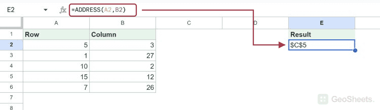
Row 5 and column 3 identify C5. With the default reference mode, ADDRESS includes dollar signs for both coordinates.
=ADDRESS(A2,B2)Result: $C$5
Choose absolute, mixed, or relative text
Mode 2 locks the row in the returned address text.
=ADDRESS(5,3,2)Result: C$5
Mode 3 locks the column instead.
=ADDRESS(5,3,3)Result: $C5
Mode 4 returns the address without dollar signs.
=ADDRESS(5,3,4)Result: C5
Use a sheet name or R1C1 notation
Pass the sheet name as the fifth argument. ADDRESS adds the single quotes needed around Q1 Sales; do not add another pair yourself.
=ADDRESS(2,1,1,TRUE,"Q1 Sales")Result: ‘Q1 Sales’!$A$2
Set the fourth argument to FALSE for R1C1 notation. This example uses absolute row and column numbers.
=ADDRESS(5,3,1,FALSE)Result: R5C3
Get the value at a generated address
ADDRESS constructs $B$4, then INDIRECT reads B4. In this example B4 contains the column number 2.
=INDIRECT(ADDRESS(4,2))Result: 2
Find the address of the largest value
MATCH locates the largest number in B2:B6. Adding ROW(B2)-1 converts that relative position into the worksheet row before ADDRESS builds the result.
=ADDRESS(MATCH(MAX(B2:B6),B2:B6,0)+ROW(B2)-1,COLUMN(B2))Result: $B$3
Convert a column number to its letter
Build a relative address in row 1, then remove its digits. Column 27 becomes AA, which answers a common column-letter lookup task.
=REGEXREPLACE(ADDRESS(1,27,4),"[0-9]","")Result: AA
Generate addresses for several rows
ARRAYFORMULA applies ADDRESS to each pair of row and column numbers. Leave enough empty cells below the formula for the five results.
=ARRAYFORMULA(ADDRESS(A2:A6,B2:B6))| $C$5 |
| $AA$1 |
| $B$10 |
| $L$15 |
| $Z$7 |
Other Google Sheets articles you may also like