COLUMNS Function in Google Sheets

If you want to know how many columns a range spans, the COLUMNS function in Google Sheets gives you that count in one shot.

It is also handy as a helper inside bigger formulas, where you need the column count of a range without hardcoding a number.

In this article, I’ll walk you through four practical examples that show where COLUMNS earns its keep, including a couple of clever pairings with INDEX, ROWS, and INDIRECT.

COLUMNS Function Syntax in Google Sheets

COLUMNS takes a single argument.

=COLUMNS(range)

• range: the range or array whose column count you want. This can be a literal range like A1:E10, a named range, or a reference returned by another function.

COLUMNS always returns a positive integer. The row count of the range does not affect the answer.

When to Use COLUMNS Function

• Count how many columns a range or table spans without manually inspecting the sheet.
• Find out how many fields a dataset has by pointing COLUMNS at the header row.
• Feed a column index into INDEX so your lookup automatically picks the last column.
• Multiply ROWS by COLUMNS to get the total number of cells inside a range.
• Keep formulas resilient when the underlying range grows or shrinks.

Example 1: Count the columns in any range

Let’s start with the most straightforward use case. You have a list of ranges written as text, and you want to know how many columns each one spans.

Below is a small table with five range references typed into column A.

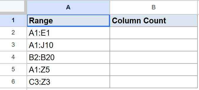
The goal is to return the column count for each range in column B.

Here is the formula:

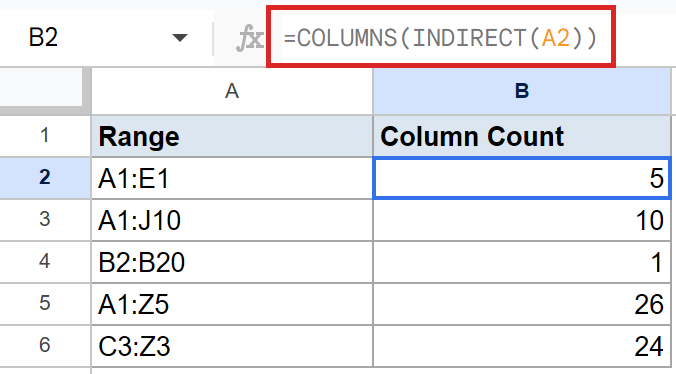
=COLUMNS(INDIRECT(A2))

Put it in B2 and fill it down through B6. INDIRECT converts the text in column A into a live range reference, and COLUMNS then counts its columns.

The results follow the range shapes:

• A1:E1 spans 5 columns (A through E).
• A1:J10 spans 10 columns (A through J), and the row count does not matter.
• B2:B20 spans 1 column, since both ends sit in column B.
• A1:Z5 spans 26 columns (A through Z).
• C3:Z3 spans 24 columns (C through Z).

Pro Tip: If you swap COLUMNS for ROWS, you get the row count of the same range instead. ROWS is the row-side equivalent and is often used alongside COLUMNS in the same formula.

Example 2: Count the columns in a dataset header row

When you inherit a dataset, the quickest way to see how many fields it has is to point COLUMNS at the header row. No need to count headers by eye.

Below is a small contacts table with five header fields and three data rows.

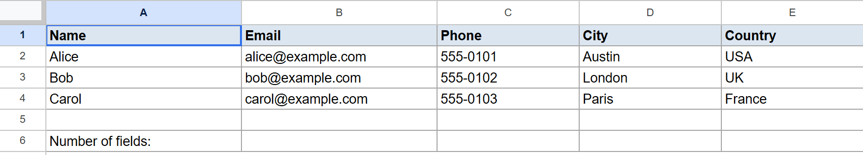
The goal is to show the number of fields in the dataset in cell B6.

Here is the formula:

=COLUMNS(A1:E1)

Put it in B6.

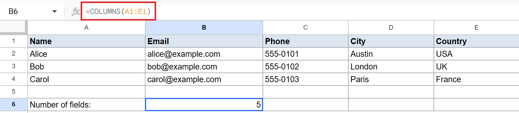
The formula returns 5, since the header range A1:E1 covers Name, Email, Phone, City, and Country.

If you later add a sixth field in column F and extend the formula to =COLUMNS(A1:F1), the count updates to 6.

For tables that grow dynamically, point COLUMNS at the entire header row (for example =COLUMNS(1:1) after trimming the blank columns) so you don’t have to revisit the formula.

Pro Tip: When you have a fully populated header row with no blanks to the right, =COUNTA(1:1) gives you the same count without needing to know the end column. COLUMNS is better when you want to pin the range explicitly.

Example 3: Grab the value in the last column of a row with INDEX and COLUMNS

This is where COLUMNS starts pulling its weight inside other formulas. INDEX needs a column index, and you can feed it COLUMNS(range) so it always points at the rightmost column, even when the table grows.

Below is a small monthly sales table with regions in column A and four months across columns B through E.

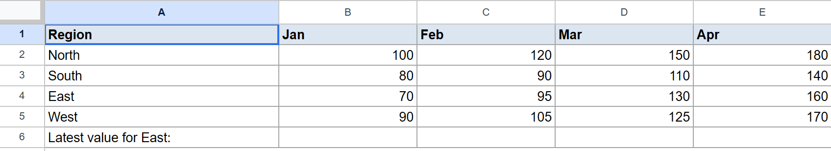
The goal is to return the latest value for the East region (row 3 of the data, which is the third entry in the data range) without manually picking the last month’s column.

Here is the formula:

=INDEX(B2:E5,3,COLUMNS(B2:E5))

Put it in B6.

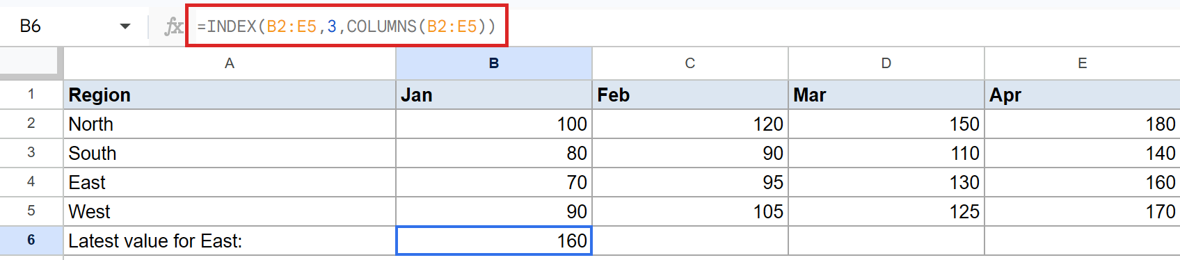
The formula returns 160, which is East’s April value.

How this formula works:

• COLUMNS(B2:E5) counts the columns in the data range and returns 4.
• INDEX(B2:E5, 3, 4) then fetches the value at the third row and fourth column of that range, which is row 4 column E in the sheet.
• If you extend the data range to include May (B2:F5), the column count becomes 5 and INDEX shifts to grab May’s value instead. You don’t have to edit the column index by hand.

Pro Tip: If you want the last value for a different region, replace the 3 with a MATCH on the region name: =INDEX(B2:E5, MATCH("East", A2:A5, 0), COLUMNS(B2:E5)). That makes both the row and the column dynamic.

Example 4: Count total cells in a range with ROWS and COLUMNS

Sometimes you want to know the total cell count of a range, for sanity-checking or for budgeting how much data you’re working with. Multiply ROWS by COLUMNS and you have it.

Below is a small table of range references in column A, with placeholder columns for row count, column count, and total cells.

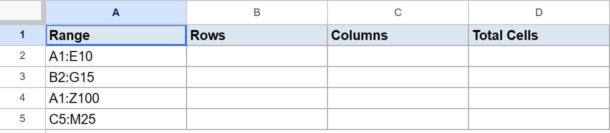
The goal is to compute the total number of cells in each range without manually picking the dimensions.

Here is the formula:

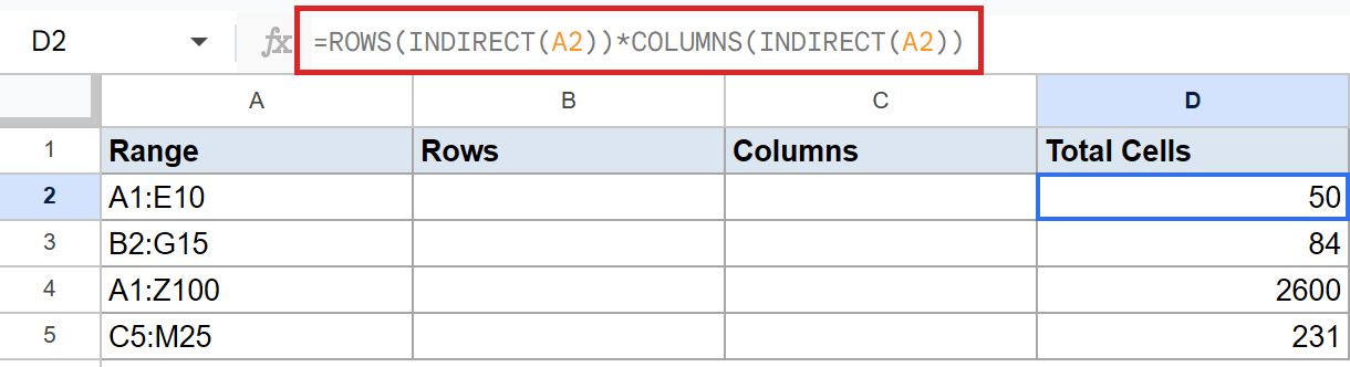
=ROWS(INDIRECT(A2))*COLUMNS(INDIRECT(A2))

Put it in D2 and fill it down through D5.

Each row gets its own total:

• A1:E10 has 10 rows and 5 columns, so 50 cells.
• B2:G15 has 14 rows and 6 columns, so 84 cells.
• A1:Z100 has 100 rows and 26 columns, so 2,600 cells.
• C5:M25 has 21 rows and 11 columns, so 231 cells.

Pro Tip: If you already know the range as a real reference (not text), drop INDIRECT and write =ROWS(B2:G15)*COLUMNS(B2:G15) directly. INDIRECT is only needed when the range is stored as text in another cell.

Tips & Common Mistakes

• Don’t confuse COLUMNS with COLUMN. COLUMNS returns the column count of a range. COLUMN returns the column position of a single cell (for example =COLUMN(C5) returns 3). The plural-versus-singular swap is the most common slip.
• Pass a range, not a single cell. =COLUMNS(A2) returns 1, which is rarely what you want. COLUMNS only earns its keep when the argument is a range or an array, so make sure both ends of the range are present.
• Pair with ROWS for total cells. ROWS counts rows the same way COLUMNS counts columns. Multiplying them gives you the cell count without hardcoding the dimensions, which is useful when ranges grow dynamically.

COLUMNS is one of those small functions that sits quietly in the background of bigger formulas. It rarely gets the spotlight on its own.

The moment you pair it with INDEX, ROWS, or a dynamic range, it makes the formula self-adjusting and saves you from rewriting numbers every time the data shape changes.

List of All Google Sheets Functions

Related Excel Functions:

• COLUMN Function in Google Sheets