A pivot table is great for summarizing data, but pulling one specific number out of it into another cell is where people get stuck. Point a normal reference like =F5 at a pivot table and it breaks the moment the pivot reorders or grows.
The GETPIVOTDATA function solves that. It grabs a value from a pivot table by name, so the right number follows along even when the pivot changes shape.
GETPIVOTDATA Function Syntax in Google Sheets
Here is how the function is structured.
=GETPIVOTDATA(value_name, any_pivot_table_cell, [original_column, ...], [pivot_value, ...])
- value_name: The name of the summarized value, exactly as it appears in the pivot table, in quotes. For a sum of a Sales column this is usually
"SUM of Sales". - any_pivot_table_cell: A reference to any cell inside the pivot table. The top-left corner is the safest choice.
- original_column, pivot_value: Optional pairs. The first is a field name, the second is the item you want from it (like
"Region","East"). Add more pairs to narrow the result further.
When to Use GETPIVOTDATA Function
- You want to pull a single number from a pivot table into a summary cell or dashboard.
- You need a reference that stays correct even when the pivot table reorders or adds rows.
- You want a small lookup where someone picks a category and sees its total.
- You want to avoid direct cell references like
=F5that break when the pivot shifts.
Example 1: Pull the Grand Total From a Pivot Table
Let’s start with the simplest case.
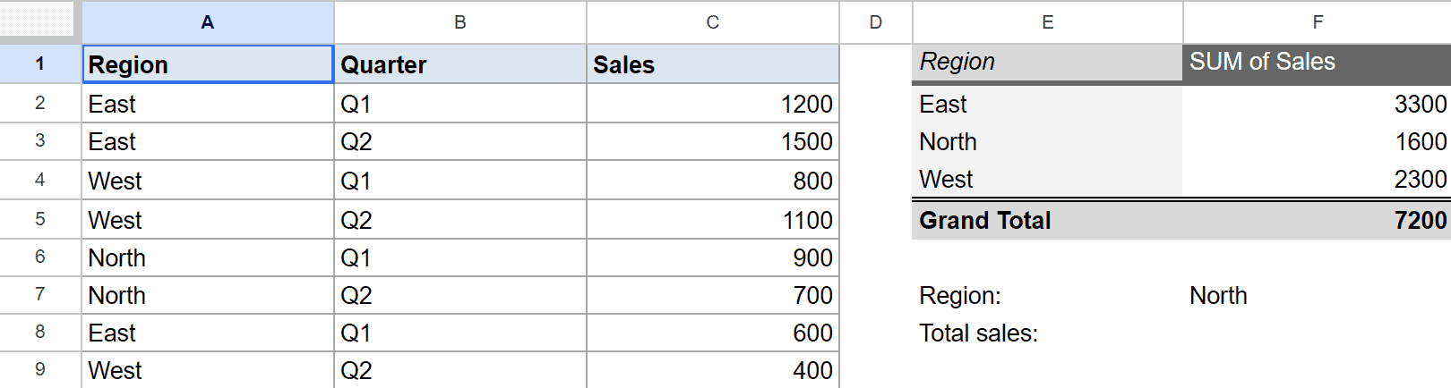
Below is the dataset. Column A has the region, column B the quarter, and column C the sales for each order. To the right is a pivot table that totals sales by region.
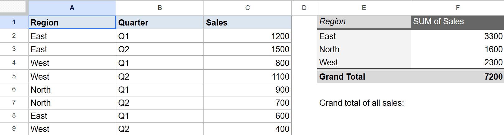
I want to pull the overall total of every sale out of that pivot table.
Here is the formula:
=GETPIVOTDATA("SUM of Sales", E1)
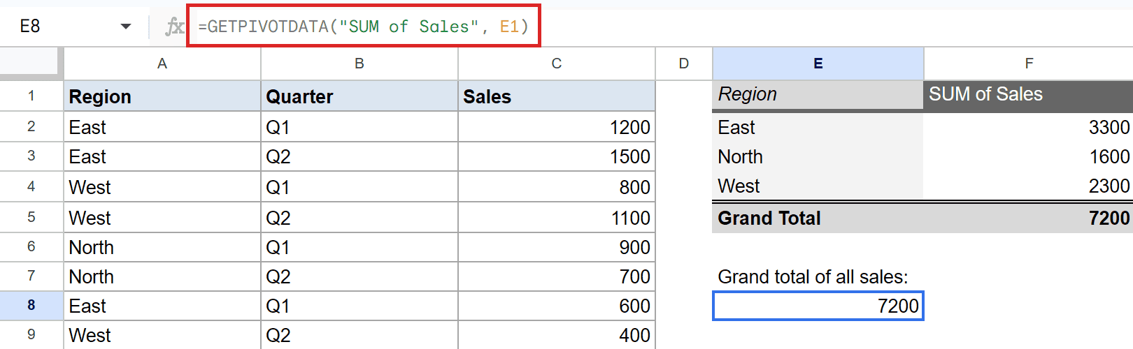
GETPIVOTDATA needs two things at a minimum. The name of the value you want, and a cell that sits inside the pivot table.
Here "SUM of Sales" is the label Google Sheets gave the totals column, and E1 points at the pivot. With no extra criteria, it returns the grand total, which is 7200.
Pro Tip: The second argument can be any cell inside the pivot table, not just E1. The top-left corner is the safest pick because it never moves when the pivot grows.
Example 2: Get the Total for One Region
Now let’s narrow it down to a single region.
Below is the same sales data with the same pivot table summarizing sales by region.
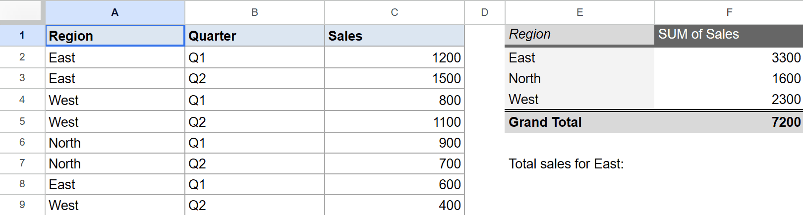
This time I only want the total sales for the East region.
Here is the formula:
=GETPIVOTDATA("SUM of Sales", E1, "Region", "East")
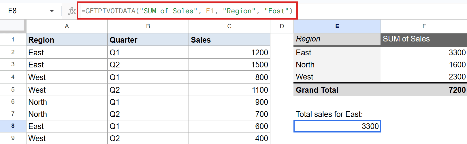
The extra pair is what does the work. "Region" is the field, and "East" is the item inside it that you want.
The function looks up the East row in the pivot table and returns its total, which is 3300.
Pro Tip: The field name must match your source header exactly. If your column is called Region, write “Region”, not “Regions” or “region group”.
Example 3: Pull a Value by Row and Column
Pivot tables often break data down two ways at once. GETPIVOTDATA can target a single cell in that grid.
Below the pivot table now shows regions down the side and quarters across the top, so every cell is one region in one quarter.
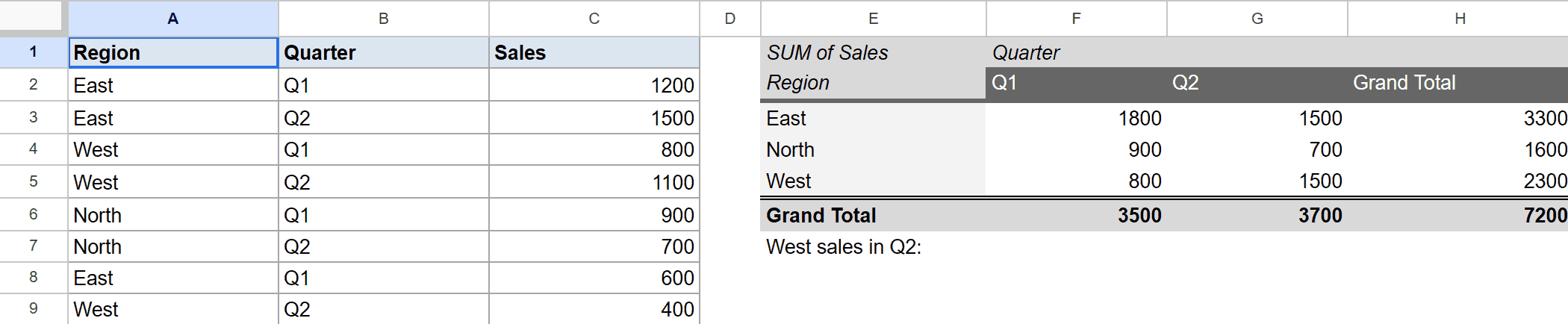
I want the West region’s sales in Q2 specifically.
Here is the formula:
=GETPIVOTDATA("SUM of Sales", E1, "Region", "West", "Quarter", "Q2")
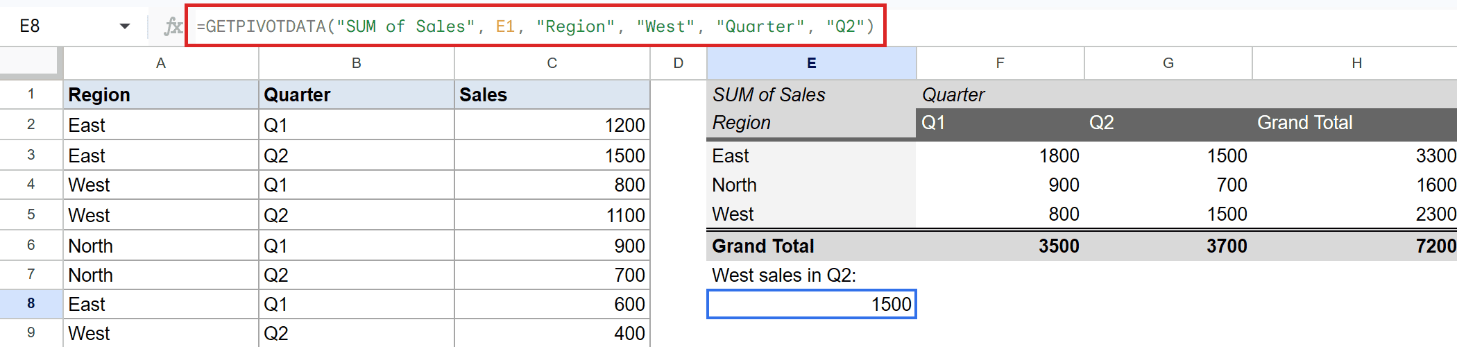
You stack a second pair to pin both a row and a column. The first pair picks the West row, the second picks the Q2 column.
Where they cross is the value the function returns, which is 1500. You can keep adding pairs for any field in the pivot.
Example 4: Read a Count Instead of a Sum
The value name changes when the pivot summarizes data a different way. This trips a lot of people up.
Below the pivot table counts the orders in each region instead of adding up sales. Notice the header now reads COUNTA of Sales.
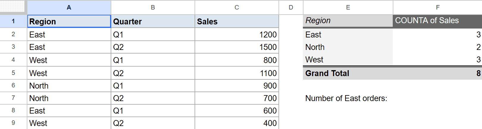
I want to know how many orders came from the East region.
Here is the formula:
=GETPIVOTDATA("COUNTA of Sales", E1, "Region", "East")
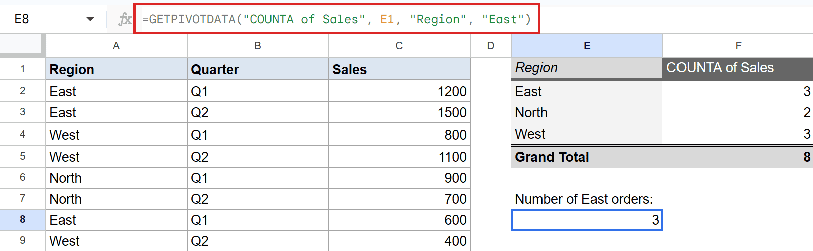
The criteria pair is the same as before. The only change is the value name.
Because the pivot counts rather than sums, the label is "COUNTA of Sales". East has three orders, so the function returns 3.
Pro Tip: Not sure of the exact value name? Click the totals cell in your pivot table and read the header text above it. Copy that text into the first argument word for word.
Example 5: Make the Lookup Dynamic With a Cell Reference
Hardcoding “East” or “West” is fine, but you can make the formula respond to whatever someone types.
Below there is an input cell in F7 holding a region name, with the pivot table on the right.
I want the total to update automatically based on the region in F7.
Here is the formula:
=GETPIVOTDATA("SUM of Sales", E1, "Region", F7)
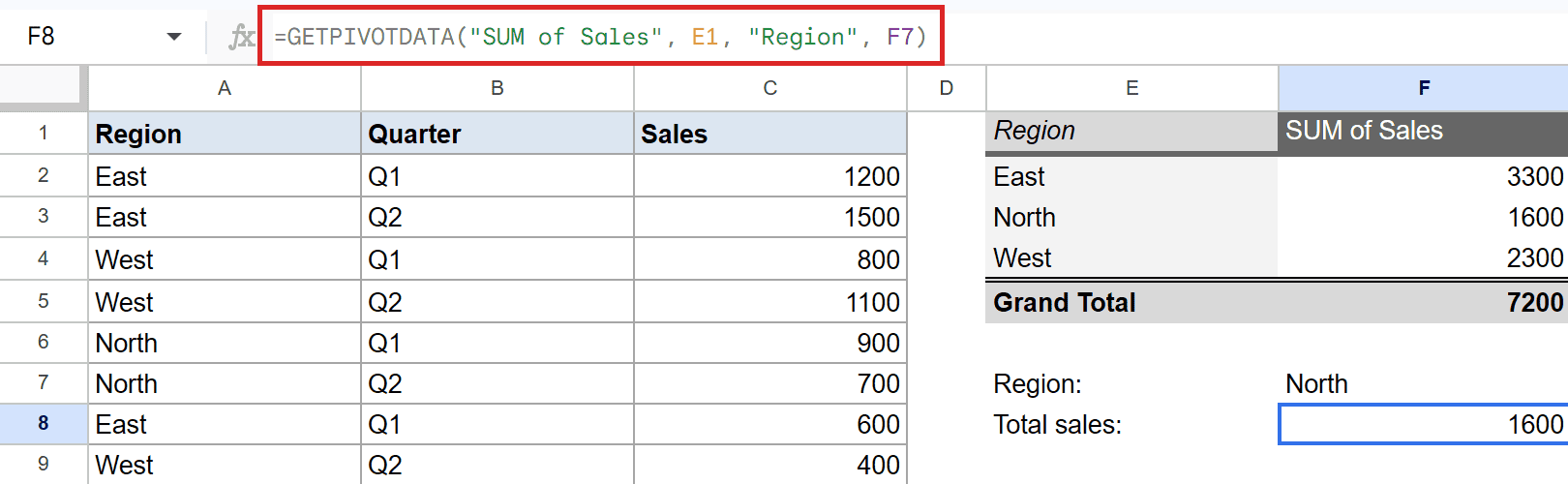
Instead of typing the region into the formula, you point the pair at cell F7. Right now F7 holds North, so the function returns 1600.
Change F7 to East or West and the total updates on its own. Pair this with a drop-down list in F7 and you have a tidy little lookup.
Pro Tip: GETPIVOTDATA only reads from a pivot table. If your numbers sit in a plain table instead, a lookup function like HLOOKUP is the better tool for pulling out a matching value.
Tips & Common Mistakes
- Match the value name exactly. The first argument has to mirror the pivot label, including the SUM of or COUNTA of prefix. Copy it straight from the pivot table to be safe.
- The value must be visible in the pivot. GETPIVOTDATA can only read what the pivot actually shows. Ask for a region that is filtered out or collapsed and you get a #REF error.
- Watch your field and item spelling. A typo in “Region” or “East” returns an error rather than a number. The names must match the pivot, so check capitalization and extra spaces.
Wrapping It Up
GETPIVOTDATA lets you pull exact values out of a pivot table without fragile cell references. Name the value you want, point at the pivot, and add field and item pairs to zero in on a single number.
It works the same whether the pivot sums, counts, or breaks data down two ways. And once you swap a hardcoded item for a cell reference, you have a lookup that updates the moment your input changes.