If you want to strip the minus sign off a number and keep just its size, the ABS function in Google Sheets does it in one step.
ABS returns the absolute value of a number, which is its distance from zero with no regard for the sign. In this article I’ll show you how to use it with three practical examples.
ABS Function Syntax in Google Sheets
Here is how you write the ABS function.
=ABS(value)
- value – the number you want the absolute value of. This can be a number you type in, a cell reference, or the result of another calculation.
When to Use ABS Function
- Turn negative numbers into positive ones while leaving positives untouched.
- Get the size of a difference between two values regardless of which is bigger.
- Calculate error or variance where you only care about the gap, not the direction.
- Clean up data where signs are inconsistent before you sum or compare it.
Example 1: Absolute Value of a Column of Numbers
Let’s start with the most basic use, flipping negatives to positives.
Below is the dataset, a single column of mixed positive and negative numbers in A2 to A6.
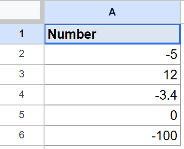
The goal is to get the magnitude of each number, dropping any minus sign.
Here is the formula:
=ABS(A2)
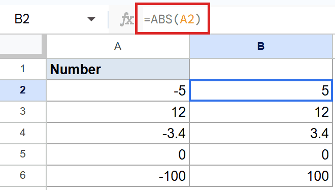
ABS returns each number’s distance from zero. So -5 becomes 5 and -3.4 becomes 3.4.
Positive numbers and zero pass through unchanged. That’s why 12 stays 12, 0 stays 0, and -100 comes back as 100.
Pro Tip: Instead of filling the formula down row by row, you can do the whole column at once with one formula: =ARRAYFORMULA(ABS(A2:A6)). Same result, just a single cell to manage.
Example 2: Magnitude of the Difference Between Two Values
A common use is finding how far apart two numbers are.
Below is the dataset, an Actual column and a Forecast column in A and B.
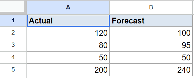
The goal is to find the size of the gap between actual and forecast, no matter which one is higher.
Here is the formula:
=ABS(A2-B2)
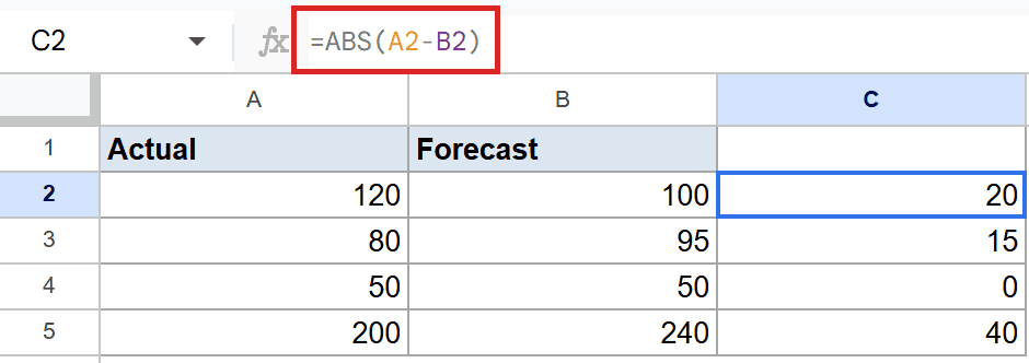
The subtraction A2-B2 can come out positive or negative depending on the order. Wrapping it in ABS forces the answer to be positive either way.
For the first row, 120 minus 100 is 20. For the second, 80 minus 95 is -15, but ABS turns that into 15. When the two match, like 50 and 50, you get 0.
Example 3: ABS Inside a Percentage Error Calculation
ABS really shines when it sits inside a bigger formula.
Below is the dataset, an Estimate column and an Actual column in A and B.
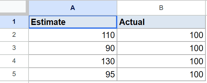
The goal is to find the absolute percentage error, the size of the miss relative to the actual value.
Here is the formula:
=ABS(A2-B2)/B2
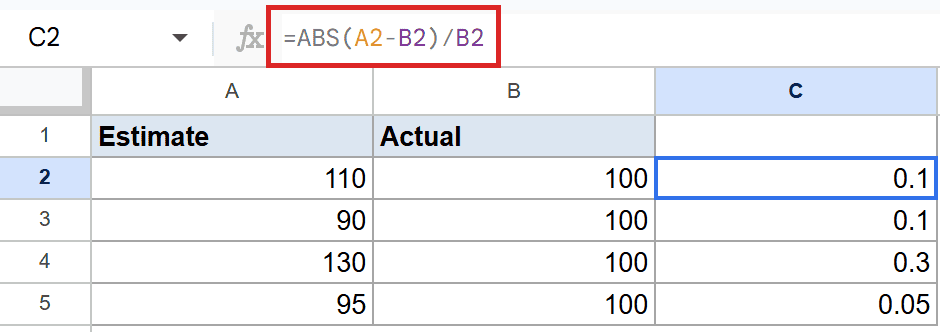
First the difference, A2-B2, is wrapped in ABS so the error is always positive. Then you divide by the actual value in B2 to get it as a fraction.
For the first row, the estimate of 110 misses the actual of 100 by 10, and 10 divided by 100 is 0.1. Format the column as a percentage and 0.1 reads as 10%.
Tips & Common Mistakes
- ABS only changes the sign, never the size. A value of 7 stays 7 and -7 also becomes 7.
- It works on any numeric input, including the result of a calculation, so you can wrap whole expressions like
ABS(A2-B2)rather than single cells. - If a cell holds text instead of a number, ABS returns a #VALUE! error. Make sure the input is numeric before applying it.
ABS is one of those functions you reach for without thinking once you know it’s there. Whether you’re cleaning up signs, measuring a gap, or building an error formula, it keeps your numbers positive.
Drop it into your own data and see how often a stray minus sign was getting in your way.