
Sometimes the data you need lives in a different Google Sheet. Copying it over by hand means it goes stale the moment the original changes.
The IMPORTRANGE function pulls a range from another spreadsheet straight into your own, and it stays linked. This tutorial walks through five practical ways to use it, starting with a plain table pull and working up to filtering the imported data with QUERY.
IMPORTRANGE Function Syntax in Google Sheets
IMPORTRANGE takes two pieces of text: where the data lives, and which range to grab.
=IMPORTRANGE(spreadsheet_url, range_string)
- spreadsheet_url: the full URL (or just the key) of the source spreadsheet, wrapped in quotes.
- range_string: the tab name and range you want, like
"Sales!A1:C7", also in quotes.
The result spills into the cells below and to the right of where you enter the formula, so make sure that space is empty.
When to Use IMPORTRANGE Function
- Pull a table from another file into the sheet you are working in.
- Build a dashboard that reads from data owned by other people or teams.
- Combine data that is split across several spreadsheets.
- Keep a live link so edits in the source flow through to your sheet automatically.
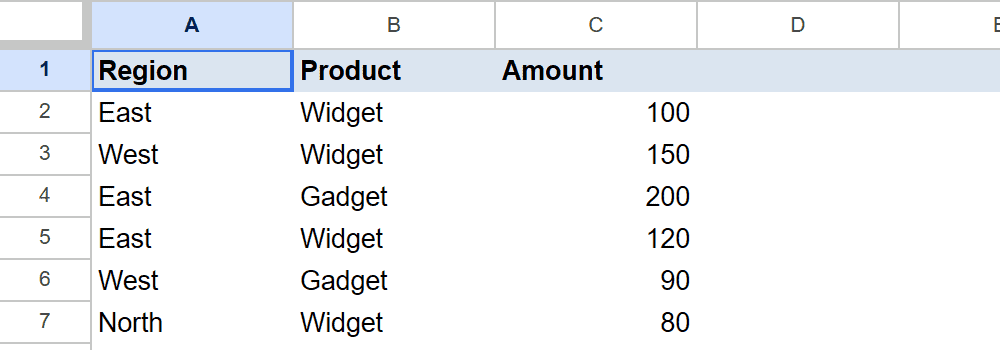
Throughout the examples below, we pull from a source sheet that holds a simple sales log. Here is what that source data looks like.
Example 1: Import an Entire Range
Let’s start by pulling the whole table into a fresh sheet.
We want every row and column from the Sales tab, cells A1 through C7.
Here is the formula:
=IMPORTRANGE("https://docs.google.com/spreadsheets/d/1L--xmJPhL-5jQ0S3MoyxDU20zx7gvb4w5na2uMKn8mQ/edit", "Sales!A1:C7")
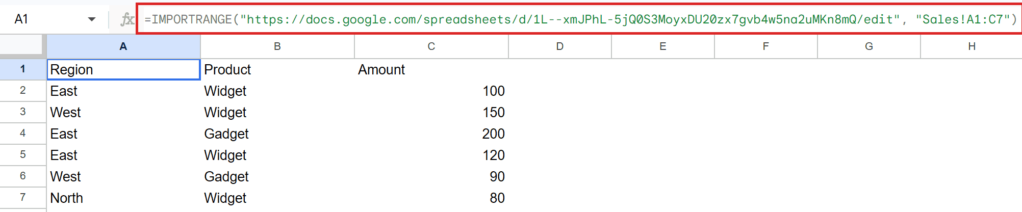
The whole block lands in your sheet, headers and all. You only type the formula once in the top-left cell, and the rest spills out from there.
Pro Tip: The first time you link two sheets, the cell shows #REF! with a “You need to connect these sheets” message. Click the cell, then click Allow access. You only do this once per source sheet.
Example 2: Import a Single Column
You don’t have to grab the whole table. You can pull just one column.
Here we want only the Amount column, cells C1 through C7.
Here is the formula:
=IMPORTRANGE("https://docs.google.com/spreadsheets/d/1L--xmJPhL-5jQ0S3MoyxDU20zx7gvb4w5na2uMKn8mQ/edit", "Sales!C1:C7")
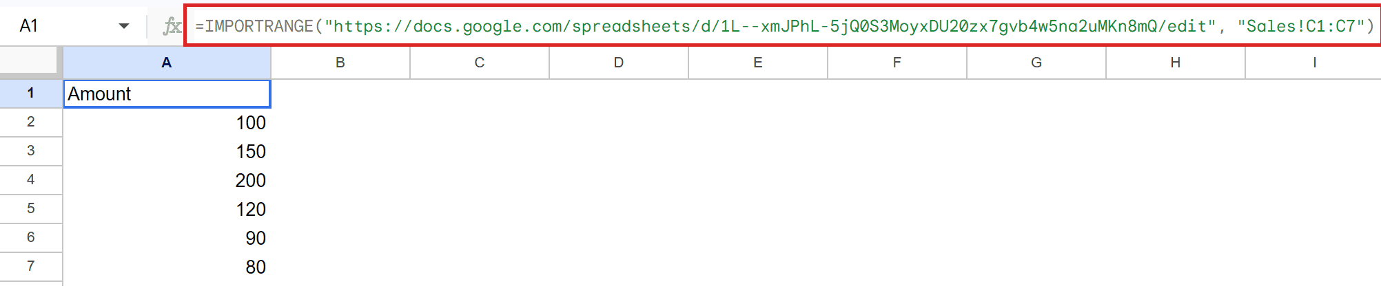
Only the Amount values come across. The range string controls exactly what gets imported, so narrow it down to what you actually need.
Example 3: Reference the Source by Its Key
The first argument doesn’t have to be the full URL. Every Google Sheet has a unique key in its address, and IMPORTRANGE accepts that too.
The key is the long string between /d/ and /edit in the spreadsheet URL.
Here is the formula:
=IMPORTRANGE("1L--xmJPhL-5jQ0S3MoyxDU20zx7gvb4w5na2uMKn8mQ", "Sales!A1:C7")
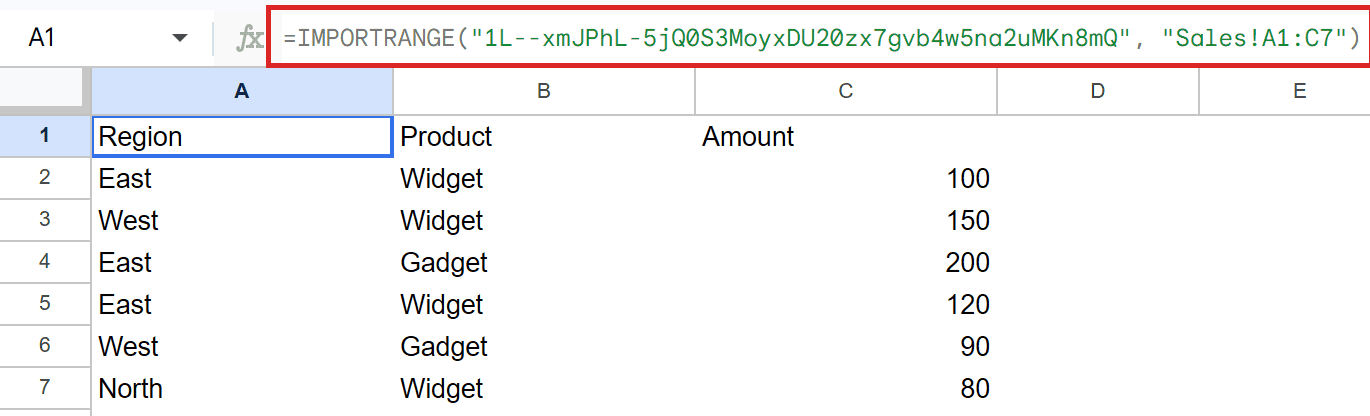
Same table, shorter formula. Both forms work, so use whichever you find easier to read.
Example 4: Total Imported Numbers With SUM
IMPORTRANGE returns a normal range, which means other functions can work on it directly.
Say we want the total of the imported amounts without first landing them in cells. We wrap IMPORTRANGE inside SUM.
Here is the formula:
=SUM(IMPORTRANGE("https://docs.google.com/spreadsheets/d/1L--xmJPhL-5jQ0S3MoyxDU20zx7gvb4w5na2uMKn8mQ/edit", "Sales!C2:C7"))

The imported amounts add up to a single total in one cell. The same trick works with AVERAGE, COUNT, MAX, and most other functions.
Pro Tip: You have to authorize the connection before a wrapped formula like this will work. If SUM returns #REF!, run a plain IMPORTRANGE in a spare cell first, click Allow access, then come back.
Example 5: Filter Imported Data With QUERY
You can also slice the imported data as it comes in, instead of bringing over everything.
Here we want only the Widget rows, showing the Region and Amount. QUERY handles the filtering on top of the imported range.
Here is the formula:
=QUERY(IMPORTRANGE("https://docs.google.com/spreadsheets/d/1L--xmJPhL-5jQ0S3MoyxDU20zx7gvb4w5na2uMKn8mQ/edit", "Sales!A1:C7"), "select Col1, Col3 where Col2 = 'Widget'", 1)

How this formula works:
- IMPORTRANGE pulls the full Sales table into QUERY.
- Inside QUERY, the columns are referenced as Col1, Col2, Col3 instead of A, B, C.
select Col1, Col3 where Col2 = 'Widget'keeps the Region and Amount for Widget rows only.- The final
1tells QUERY the imported data has one header row.
Tips & Common Mistakes
- Authorize the connection first. The most common IMPORTRANGE problem is a #REF! error on a brand new link. Click the cell and choose Allow access. Until you do, nothing imports.
- Quote both arguments. Both the URL (or key) and the range string must be inside double quotes. Leaving the quotes off the range is an easy mistake that breaks the formula.
- Leave room for the result. IMPORTRANGE spills, so if there is anything in the cells where the data would land, you get a #REF! that says the result would overwrite data. Clear that space or move the formula.
IMPORTRANGE is the cleanest way to keep data flowing between Google Sheets without copy and paste. Start with a plain range pull, authorize the link once, then layer SUM or QUERY on top when you need totals or filtered views.
List of All Google Sheets Functions
Related Google Sheets Functions / Articles: