FV Function in Google Sheets

If you want to know what an investment will be worth after a stretch of regular contributions or a lump sum sitting and compounding, the FV function in Google Sheets is the tool for the job. You feed it a rate, a number of periods, a payment, and a starting balance, and it returns the future value.

In this article, I’ll walk through four practical examples covering monthly savings, one-time deposits, mixed contributions, and a parameter-driven setup.

FV Function Syntax in Google Sheets

Here is how you write the FV function.

=FV(rate, number_of_periods, payment_amount, [present_value], [end_or_beginning])

• rate – the interest rate per period. For monthly compounding, divide the annual rate by 12.
• number_of_periods – the total number of payment periods. For a 10-year monthly plan, this is 12*10.
• payment_amount – the payment made each period. Money you put IN is negative, money you take OUT is positive.
• present_value – optional. The starting balance. Same sign convention as payment.
• end_or_beginning – optional. 0 (default) means payments are made at the end of each period, 1 means at the start.

One thing to know upfront. FV follows a sign convention. Cash you pay IN (a deposit, a payment) is negative. Cash you get OUT (the final balance) is positive. Get the signs wrong and you’ll see a negative result where you expected a positive one.

When to Use FV Function

• Project what regular monthly savings will grow to over a set number of years.
• Estimate how much a one-time deposit will be worth after compounding for X years.
• Model an account that has both a starting balance and ongoing contributions.
• Build a what-if savings sheet driven by labeled input cells.
• Compare investment scenarios by varying the rate, periods, or contribution.

Example 1: Future Value of Monthly Savings Over 10 Years

Start with the classic savings question.

Below is the dataset, a single scenario description in A2 covering $200 a month for 10 years at 6 percent annual interest.

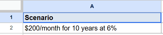
The goal is to compute what those monthly contributions grow to at the end of the 10 years.

Here is the formula:

=FV(0.06/12, 12*10, -200, 0)

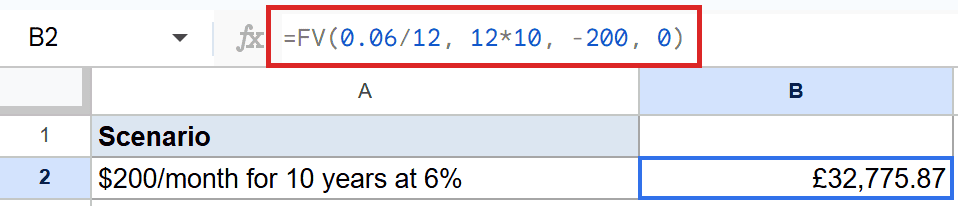
The cell lands at $32,775.87 (rounded for display). The underlying value is 32775.8693612916, which is the full float Google Sheets stores.

Here is what each argument does. 0.06/12 is the monthly rate because the payments are monthly. 12*10 is 120 months. -200 is the monthly contribution (negative because it leaves your pocket). 0 says there is no starting balance.

Pro Tip: Always match the rate period to the payment period. Monthly payments need a monthly rate (annual divided by 12). Quarterly payments need a quarterly rate (annual divided by 4). Mismatching them silently inflates or deflates the answer.

Example 2: Future Value of a One-Time Deposit

No monthly payments, just a lump sum sitting in an account.

Below is the dataset, a single scenario in A2 covering a $10,000 deposit for 10 years at 5 percent annual interest.

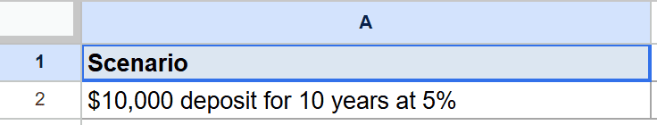
The goal is to see what the $10,000 grows to after 10 years.

Here is the formula:

=FV(0.05, 10, 0, -10000)

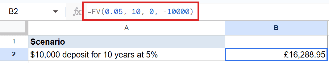
The cell lands at $16,288.95 (full value 16288.94626777442). Because the rate is annual and the period is years, no division by 12 is needed. The payment is 0 since there are no contributions. The present value of -10000 is the starting deposit, negative because it left your pocket.

This is the simplest FV scenario. The final value compounds purely from the starting balance.

Example 3: Combine a Starting Balance With Monthly Contributions

Most real accounts have both a balance and ongoing deposits.

Below is the dataset, a single scenario in A2 covering a $5,000 starting balance plus $300 a month for 20 years at 7 percent.

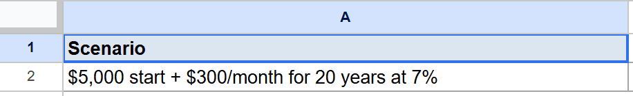
The goal is to combine both the lump sum and the monthly stream into one final value.

Here is the formula:

=FV(0.07/12, 12*20, -300, -5000)

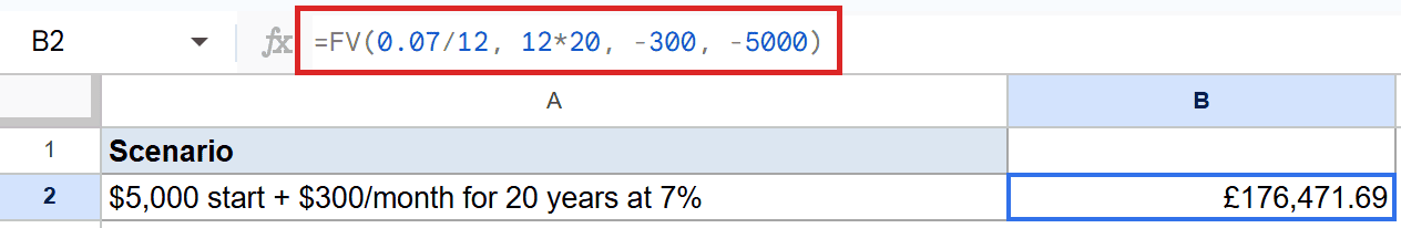
The cell lands at $176,471.69 (full value 176471.69219256623). Both the $300 monthly payment and the $5,000 starting balance are negative because they are money you put IN. FV compounds both pieces together and gives you the combined future balance.

This pattern is the one most people actually want. A starting amount, regular contributions, a long horizon.

Example 4: FV Driven by Parameter Cells

For a what-if sheet, point FV at named input cells instead of hard-coded numbers.

Below is the dataset, with the annual rate in A2, the number of periods in B2, the payment in C2, and the present value in D2.

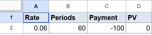
The goal is to read every argument from the input cells so changing the inputs auto-updates the answer.

Here is the formula:

=FV(A2/12, B2, C2, D2)

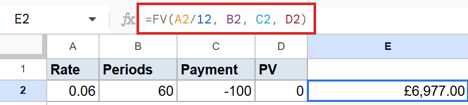
The cell lands at $6,977.00 (full value 6977.00305098615). Notice that A2/12 divides the annual rate (6 percent in A2) by 12 right inside the formula. That way the input cell stays the headline annual rate and the formula handles the monthly conversion.

Want to model a different scenario? Change the value in A2 from 0.06 to 0.08 and watch every dependent cell update. That is the whole point of a parameter-driven sheet.

Tips & Common Mistakes

• Get the signs right – money going OUT of your pocket (deposits, payments) is negative. The FV result, which is money you would take OUT at the end, comes back positive. Flip a sign and you’ll see a negative answer.
• Match the rate to the payment period – monthly payments need annual rate / 12 and total months for periods. Mixing an annual rate with monthly periods is the most common FV bug.
• Default is end-of-period payments – the optional end_or_beginning argument is 0 by default. Set it to 1 for annuity-due style payments at the start of each period. The difference compounds over many years.

That covers projecting future values from contributions, lump sums, and combined accounts with FV. Match the rate to the payment period, keep your signs straight, and pair FV with the PMT function when you need the per-period payment instead.

List of All Google Sheets Functions

Related Google Sheets Functions / Articles:

• PMT Function in Google Sheets
• CUMIPMT Function in Google Sheets