If you want to work out the regular payment on a loan or how much to set aside each month to hit a savings goal, the PMT function in Google Sheets handles it. You give it the interest rate, the number of payments, and the amount, and it hands back the payment per period.
One thing to know up front. PMT returns a negative number because the payment is money leaving your pocket. In this article, I’ll walk you through how it works with four examples.
PMT Function Syntax in Google Sheets
Here is how the PMT function is written:
=PMT(rate, number_of_periods, present_value, [future_value], [end_or_beginning])
- rate is the interest rate for each period. For a monthly payment, divide the annual rate by 12.
- number_of_periods is the total number of payments. For monthly payments over several years, multiply the years by 12.
- present_value is the amount the payments are based on, like the loan amount you borrow today.
- future_value is optional. It’s the balance you want left at the end, which defaults to 0.
- end_or_beginning is optional. Use 0 (the default) for payments at the end of each period, or 1 for the start.
When to Use PMT Function
- Finding the monthly payment on a car loan, mortgage, or personal loan.
- Comparing how the payment changes when you shorten or extend the term.
- Working out how much to save each month to reach a target amount.
- Checking how payments shift when they’re due at the start of the period.
- Building a quick loan or savings estimate without a separate calculator.
Example 1: Monthly Payment on a Car Loan
Let’s start with the most common case, a basic monthly loan payment.
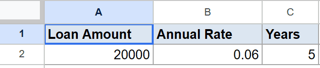
Below is the dataset. Column A holds the loan amount, column B holds the annual interest rate, and column C holds the term in years.
I want the monthly payment on a 20,000 loan at 6 percent over 5 years.
Here is the formula:
=PMT(B2/12, C2*12, A2)

The monthly payment comes to about -$386.66. I divide the annual rate by 12 to get the monthly rate, and multiply the years by 12 to get the total number of payments.
The result is negative because it’s cash going out each month. If you’d rather see it as a positive number, wrap the whole thing in ABS, or put a minus sign in front of the formula.
Pro Tip: To show the payment as a positive figure, use =ABS(PMT(B2/12, C2*12, A2)). Same payment, friendlier sign.
Example 2: See How a Shorter Term Changes It
Same loan, but let’s pay it off faster and see what happens.
Below is the dataset. The columns are the same as before, but the term in column C is now 3 years instead of 5.
I want the monthly payment on the same 20,000 loan at 6 percent, paid off in 3 years.

Here is the formula:
=PMT(B2/12, C2*12, A2)
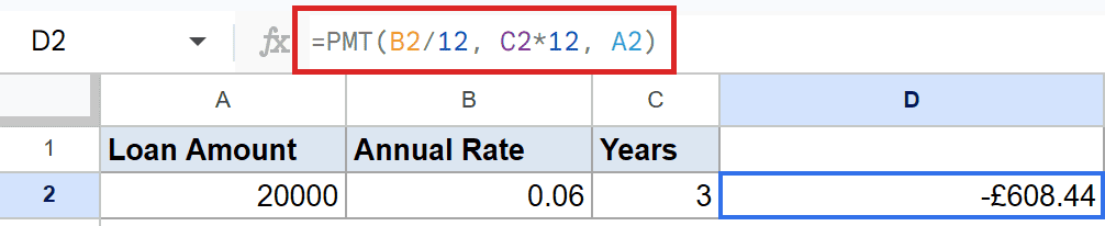
With the shorter term, the monthly payment works out to roughly -$608.44. Fewer payments means each one has to be bigger to clear the same balance.
This is a quick way to see the trade-off. A shorter term costs more each month but clears the loan sooner.
Example 3: Save Toward a Goal
PMT isn’t only for loans. You can flip it around to find how much to save.
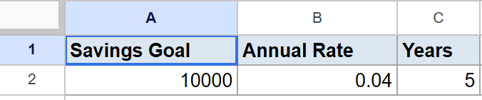
Below is the dataset. Column A holds the savings goal, column B holds the annual rate your savings earn, and column C holds the number of years.
I want to know the monthly deposit needed to reach 10,000 in 5 years at 4 percent.
Here is the formula:
=PMT(B2/12, C2*12, 0, A2)
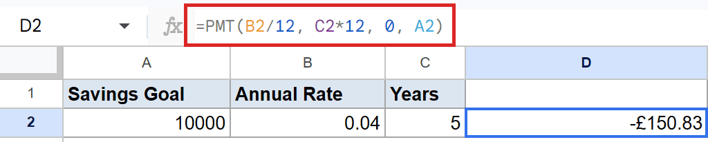
The monthly deposit lands at about -$150.83. Here the present value is 0 because you start with nothing, and the goal goes in the future_value slot as the fourth argument.
It’s negative for the same reason as before. The deposit is money you’re putting away each month, so it counts as cash leaving your account.
Example 4: Payments Due at the Start of the Period
By default PMT assumes you pay at the end of each period. Some loans charge at the start instead.
Below is the dataset. It’s the same 20,000 loan at 6 percent over 5 years from the first example.
I want the monthly payment when each payment is due at the start of the period.

Here is the formula:
=PMT(B2/12, C2*12, A2, 0, 1)
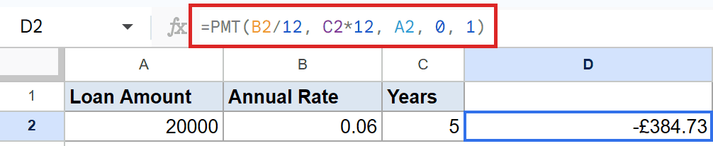
With the final argument set to 1, the payment comes to roughly -$384.73, a touch lower than the end-of-period version. Paying earlier gives the balance slightly less time to gather interest.
The fifth argument is the switch. Leave it out or set it to 0 for end-of-period, or set it to 1 for start-of-period.
Pro Tip: The future_value (4th) and end_or_beginning (5th) arguments are optional. If you only need a standard end-of-period loan payment, you can stop after present_value.
Tips & Common Mistakes
- Match the rate and periods to the same unit. For a monthly payment, the rate must be the monthly rate (annual / 12) and the periods must be in months (years * 12). Mixing an annual rate with monthly periods gives nonsense.
- The negative sign is expected. A negative result means money leaving your pocket. Wrap PMT in ABS if you want it shown as a positive number.
- Don’t forget presentvalue is required. The first three arguments (rate, periods, presentvalue) must all be present. Future value and the timing flag are the only optional ones.
That’s the PMT function in Google Sheets. You’ve seen it handle a basic loan payment, a shorter term, a savings goal, and payments due at the start of the period.
Once the rate and periods line up to the same unit, the rest falls into place.
List of All Google Sheets Functions
Related Google Sheets Functions / Articles: