
CUMIPMT totals loan interest between two payment numbers. Use a constant rate, fixed payments and a period range that matches the loan schedule.
CUMIPMT function syntax
=CUMIPMT(rate, number_of_periods, present_value, first_period, last_period, end_or_beginning)- All six arguments are required. rate is interest per payment period.
- number_of_periods: full loan term in payments; present_value: positive starting loan amount.
- first_period and last_period: beginning and end payment numbers, counted from 1.
- end_or_beginning: 0 for period-end payments, 1 for period-start payments.
Set up the example data
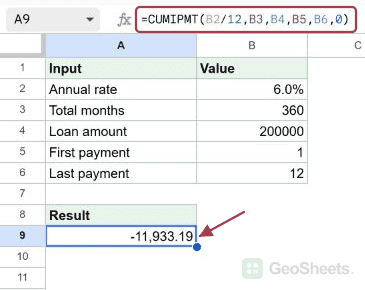
Enter this dataset starting in A1. The first row contains headings. Keep the result area separate from the source table.
| Input | Value |
|---|---|
| Annual rate | 0.06 |
| Total months | 360 |
| Loan amount | 200000 |
| First payment | 1 |
| Last payment | 12 |
Calculate interest in the first mortgage year
Enter this formula in A9. B2/12 converts the 6% annual rate to a monthly rate. Payments 1 through 12 cover the first year of this 200,000 mortgage.
=CUMIPMT(B2/12,B3,B4,B5,B6,0)Result (rounded for display): -11933.189179.
PMT calculates the full regular payment. PPMT isolates principal for one payment, while CUMIPMT sums interest over the selected window.
Total interest over an entire car loan
A 25,000 loan at 5% over 60 monthly payments has this total scheduled interest. Negate the result for a positive cost display.
=CUMIPMT(5%/12,60,25000,1,60,0)Result (rounded for display): -3306.850466.
Compare the second year of mortgage interest
Use payments 13 through 24 for the second year. The original mortgage has the same rate, term and starting amount; some principal has been repaid by this point.
=CUMIPMT(B2/12,B3,B4,13,24,0)Result (rounded for display): -11781.707028.
Change the assumptions through input cells
For another scenario, enter the labeled inputs starting at A20. The formula below uses a 250,000 mortgage at 4.5%, over 360 months, for payments 1 through 12.
| Input | Value |
|---|---|
| Annual rate | 0.045 |
| Total months | 360 |
| Loan amount | 250000 |
| First payment | 1 |
| Last payment | 12 |
=CUMIPMT(B21/12,B22,B23,B24,B25,0)Result (rounded for display): -11167.492566.
Use beginning-of-period payments
Setting the final argument to 1 changes the payment timing. The first payment is made immediately, before interest accrues, so its interest component is zero.
=CUMIPMT(B2/12,B3,B4,1,12,1)Result (rounded for display): -10878.795203.
Use whole-number period boundaries
Use integer payment numbers for clear period windows. Google documents that fractional starts round upward and fractional ends downward, so 2.8 through 4.1 includes payments 3 and 4.
=CUMIPMT(B2/12,B3,B4,2.8,4.1,0)Result (rounded for display): -1995.002539.
Check the interest for one payment
IPMT directly returns the interest for one payment. Use it when you only need payment 1, rather than a cumulative range.
=IPMT(B2/12,1,B3,B4)Result: -1000.
Other Google Sheets articles you may also like