
When you want the largest number from a range, the MAX function in Google Sheets gives it to you in a single call. Hand it a column, a 2D block, or a list of values, and you get back the biggest one.
In this article, I’ll walk through five practical MAX setups. You’ll see it on one column, across a 2D range, with literal numbers, paired with FILTER, and combined with MIN to measure a spread.
MAX Function Syntax in Google Sheets
Here is how you write the MAX function.
=MAX(value1, [value2, ...])
- value1 is the first number, range, or reference to evaluate.
- value2, … are optional extra values or ranges. You can pass as many as you need.
MAX ignores text, booleans, and empty cells. It only looks at numeric values inside whatever you hand it.
When to Use MAX Function
- Pull the highest figure out of a column of sales, scores, or measurements.
- Find the single biggest value across a full report (a 2D block of cells).
- Compare a handful of typed-in numbers without putting them in cells first.
- Combine with FILTER to get the highest value inside a subset of rows.
- Measure spread (highest minus lowest) when paired with MIN.
Example 1: Largest Score in a Single Column
Let’s start with the most common use, finding the highest value in one column.
Below is the dataset. Column A has the student name and column B has the score, across six rows.
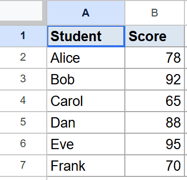
I want the largest score from the list.
Here is the formula:
=MAX(B2:B7)
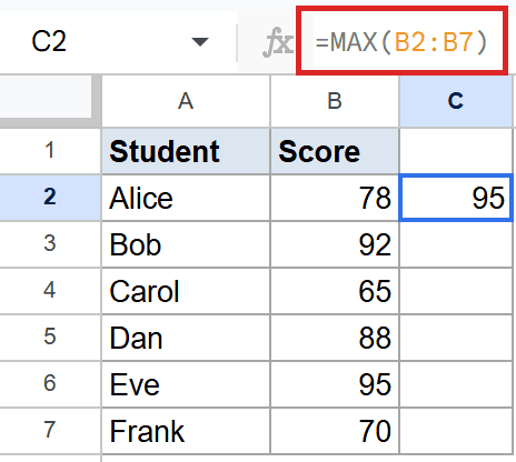
MAX walks B2:B7 and returns the biggest number, which is 95 (Eve’s score). Cells with text or blanks would be skipped, but this column is all numbers.
For a conditional version (largest score for one subject, say), reach for MAXIFS instead. Plain MAX has no built-in filter.
Example 2: Max Across a 2D Range
MAX doesn’t care if the source is one column or a whole rectangle. You can hand it a 2D block in one go.
Below is the dataset. Column A has the product, and columns B through D have Q1, Q2, and Q3 sales, across four rows.
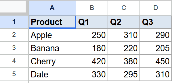
I want the single biggest value across all three quarters and all four products.
Here is the formula:
=MAX(B2:D5)
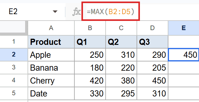
MAX scans every cell in the 4-row by 3-column block and returns the biggest one. That’s 450 (Cherry in Q3). You don’t need a helper column or a flatten step. The 2D range works directly.
If you need to know which product or quarter that came from, pair MAX with MATCH and INDEX. MAX on its own just gives you the value.
Example 3: MAX of Numbers Typed Into the Formula
You can pass numbers directly to MAX without pointing at a range at all.
Below is the setup. The formula uses four literal numbers (5, 12, 3, 8) typed inside the parentheses. No cells are referenced.

I want the largest of those four numbers.
Here is the formula:
=MAX(5, 12, 3, 8)

MAX compares all four arguments and returns 12. This form is useful when you want a quick maximum of a few known numbers, or when one of the inputs is a constant rather than a cell value (like =MAX(MyTotal, 100) to enforce a minimum floor of 100).
You can mix references and literals freely, for example =MAX(B2:B7, 80) returns whichever is larger, the biggest score in the column or the floor of 80.
Example 4: MAX of a Filtered Subset
Combining MAX with FILTER gives you a conditional maximum without writing MAXIFS.
Below is the dataset. Column A has the employee, column B has the department, and column C has the revenue, across six rows.
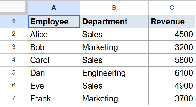
I want the largest revenue figure for employees in the Sales department.
Here is the formula:
=MAX(FILTER(C2:C7, B2:B7="Sales"))
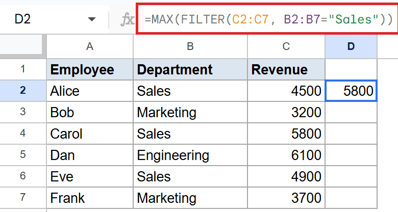
How this formula works:
- FILTER pulls only the revenue values where the department is Sales (Alice 4500, Carol 5800, Eve 4900).
- MAX wraps that filtered list and returns the largest one.
- The result is 5800 (Carol).
MAXIFS would do the same job in fewer characters, but the FILTER pattern is flexible. Swap FILTER for any range expression and you get the maximum of that subset.
Pro Tip: When the filter could be empty, MAX(FILTER(…)) throws a `#N/A` because FILTER returns nothing. Wrap the whole thing in IFERROR to fall back to 0 or a blank: `=IFERROR(MAX(FILTER(…)), 0)`.
Example 5: Range (Spread) Using MAX Minus MIN
A common analytics move is to measure the range of a dataset, which is just the maximum minus the minimum.
Below is the dataset. Column A has the day and column B has the temperature, across eight rows.
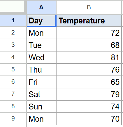
I want the spread between the hottest and coldest day.
Here is the formula:
=MAX(B2:B9)-MIN(B2:B9)
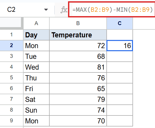
The hottest day is Wednesday at 81 and the coldest is Friday at 65. Subtracting the lower from the higher gives 16, which is the temperature range across the week.
This is a quick proxy for spread when you don’t need a full standard deviation. It only uses the two endpoints, so it can be skewed by a single outlier, but it’s instant to read.
Tips & Common Mistakes
- MAX ignores text and blanks. A cell with the word “absent” or an empty cell inside the range won’t break MAX, it just won’t count. If you want errors to propagate instead, use a stricter aggregator like AGGREGATE.
- All-text range returns 0. If every cell in the range is non-numeric, MAX returns 0, not an error. That can look like a real result. Spot-check the source if you ever see 0 from MAX on a real dataset.
- MAX has no built-in condition. For “max where department is Sales”, use MAXIFS or wrap MAX around FILTER. Plain MAX just takes the biggest from whatever you hand it.
MAX is the simplest way to find the largest number in a Google Sheets range. You’ve now seen it on a single column, a 2D range, literal arguments, a FILTER subset, and as part of a MAX-minus-MIN spread.
List of All Google Sheets Functions
Related Google Sheets Functions / Articles: