
If you need to pull just the month part out of a date, the MONTH function in Google Sheets returns it as a number from 1 to 12. You hand it a date, and you get back the month value, ready for sorting, grouping, or further calculations.
In this article, I’ll show you how to use MONTH on a list of dates, with order dates, inside SUMPRODUCT, and with nested IF for quarter labels.
MONTH Function Syntax in Google Sheets
The MONTH function reads a date and returns the month component as an integer between 1 and 12.
=MONTH(date)
- date is the date you want to read the month from. It should be a real date value or a cell holding a date, not plain text. If you have a text date, wrap it in DATEVALUE function first.
When to Use MONTH Function
- Pull the month out of a date column so you can sort or group by month.
- Total sales, expenses, or any metric for one specific month of the year.
- Tag dates with a quarter label by reading the month and bucketing it.
- Build a pivot-style breakdown without using a pivot table.
- Drive conditional formatting that highlights rows from a chosen month.
Example 1: Pull the Month Number From a Date Column
Let’s start with the simplest job, reading the month out of each date.
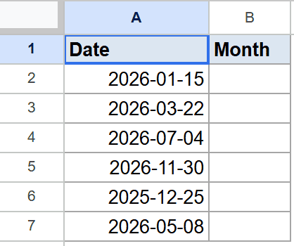
Below is the dataset. Column A has six dates spread across 2025 and 2026.
I want the month number for each date in column B.
Here is the formula:
=MONTH(A2)
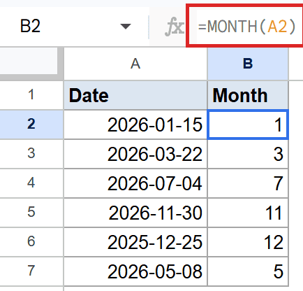
MONTH reads each date and gives back the month part as a plain integer. January becomes 1, March becomes 3, July becomes 7, November becomes 11, December becomes 12, and May becomes 5.
The day of the month and the year don’t change the result. MONTH only looks at the month slot.
Pro Tip: If you want the full month name instead of the number, use TEXT(A2, “mmmm”). That returns “January”, “March”, and so on, which is often friendlier for charts and reports.
Example 2: Extract Month Numbers From Order Dates
The same formula works no matter what years your dates span.
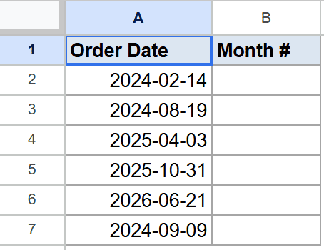
Below is the dataset. Column A has six order dates across 2024, 2025, and 2026.
I want column B to show the month number, regardless of the year.
Here is the formula:
=MONTH(A2)
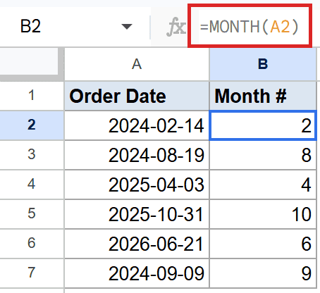
MONTH ignores the year completely. A February 2024 date and a February 2026 date both come back as 2. The output column reads 2, 8, 4, 10, 6, and 9 for the six order dates.
This is useful when you want to group orders by month across many years, like seeing which months tend to be busiest regardless of when they happened.
Example 3: Total Sales for a Single Month
MONTH gets useful when you combine it with SUMIFS function style aggregations. Here we’ll use SUMPRODUCT.
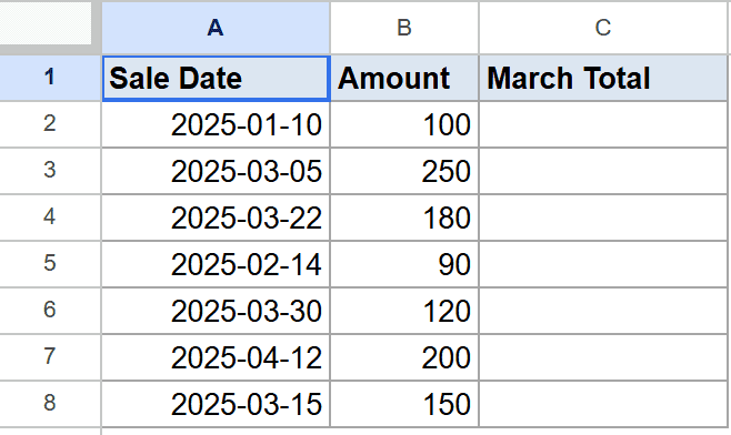
Below is the dataset. Column A has seven sale dates from January through April 2025, and column B has the amount for each sale.
I want the total of every sale that happened in March.
Here is the formula:
=SUMPRODUCT((MONTH(A2:A8)=3)*B2:B8)
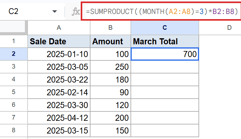
Here’s how this formula works:
- MONTH(A2:A8) returns the month for each date in the range.
- The comparison
=3turns that list into TRUE or FALSE values, one per row. - Multiplying by B2:B8 keeps only the March amounts and zeros out the rest.
- SUMPRODUCT adds them up, giving the March total of 700.
The four March rows are 250, 180, 120, and 150, which add up to the SUMPRODUCT total. The other months drop out because their TRUE/FALSE check is FALSE, which counts as zero in the multiplication.
Example 4: Label Each Date With Its Quarter
Nested IF formulas can read the month number and label the row with its quarter.
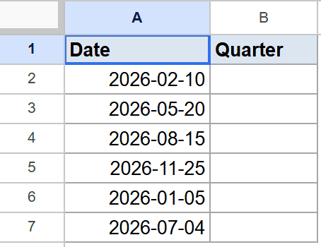
Below is the dataset. Column A has six dates and column B is where the quarter label goes.
I want Q1 through Q4 in column B, based on which quarter the date falls into.
Here is the formula:
=IF(MONTH(A2)<=3,"Q1",IF(MONTH(A2)<=6,"Q2",IF(MONTH(A2)<=9,"Q3","Q4")))
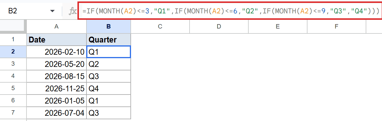
The formula reads each date’s month and walks through three checks. Months 1 to 3 get Q1, months 4 to 6 get Q2, months 7 to 9 get Q3, and anything else is Q4.
The output column reads Q1, Q2, Q3, Q4, Q1, and Q3 for the six dates. A shorter alternative is =ROUNDUP(MONTH(A2)/3,0) paired with a quarter prefix if you’d rather skip the nested IFs.
Tips & Common Mistakes
- MONTH needs a real date, not a text string. If your date is stored as text, MONTH will throw #VALUE!. Wrap text dates in DATEVALUE first, like
=MONTH(DATEVALUE(A2)), or fix the column format. - MONTH always returns a number from 1 to 12. For the full name like “January”, switch to TEXT(date, “mmmm”). For the short form, use TEXT(date, “mmm”).
- Reading the month from a blank cell returns 12. Google Sheets treats an empty cell as the serial number zero, which lands on December 30, 1899. Filter out blanks before applying MONTH if that matters for your totals.
MONTH is one of those small date functions you end up using constantly once you know it’s there.
You’ve now seen it reading dates straight, working across years, totaling a single month with SUMPRODUCT, and driving quarter labels with nested IF. That covers most of what you’ll need it for.
List of All Google Sheets Functions
Related Google Sheets Functions / Articles: