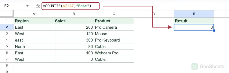
When you need to know how many cells in a range meet one condition, COUNTIF is the function to reach for. It counts matches without making you scroll through the data by hand.
This guide walks through five examples, from exact text matches to wildcards and a criteria list, so you can pick the pattern that fits your data.
COUNTIF Function Syntax in Google Sheets
Here is how the COUNTIF function is structured.
=COUNTIF(range, criterion)
- range is the group of cells you want to check.
- criterion is the condition a cell has to meet to get counted. It can be text, a number, a comparison like
">100", or a wildcard pattern.
When to Use COUNTIF Function
- Counting how many times a specific label or category shows up in a column.
- Tallying values above or below a threshold, like sales over 100.
- Finding how many entries contain a word using a wildcard.
- Building a quick frequency summary next to your data.
Example 1: Count Exact Text Matches
Let’s start with the most common job, counting how often one value appears.
Below is the dataset with an Order column in A and a Region column in B, holding six orders tagged East, West, or South.

I want to count how many orders came from the East region.
Here is the formula:
=COUNTIF(B2:B7, "East")

COUNTIF scans B2:B7 and counts every cell that equals East. There are three of them, so the formula returns 3.
The criterion sits in quotes because it is text. Numbers and cell references do not need quotes, but plain text does.
Example 2: Count Values Above a Number
Text is not the only thing COUNTIF handles. It works with number comparisons too.
Below is the dataset with a Rep column in A and a Sales column in B for five reps.

I want to count how many reps sold more than 100.
Here is the formula:
=COUNTIF(B2:B6, ">100")

The >100 part tells COUNTIF to count only values greater than 100. Alice, Carlos, and Evan clear that bar, so the result is 3.
The comparison operator and the number both go inside one set of quotes. This trips up a lot of people who try to leave the number outside.
Pro Tip: You can use any comparison operator here, including `>=`, `<=`, and `<>` for not equal. For example, `”<>0″` counts every cell that is not zero.
Example 3: Count Partial Matches with Wildcards
Sometimes you want to count cells that contain a word rather than match it exactly.
Below is the dataset with a SKU column in A and a Product column in B, listing five product names.

I want to count how many products have the word Pro anywhere in the name.
Here is the formula:
=COUNTIF(B2:B6, "*Pro*")

The asterisk is a wildcard that stands for any number of characters. Wrapping Pro in asterisks counts any cell with Pro somewhere inside it.
That matches Pro Camera, Pro Keyboard, and Webcam Pro, so the formula returns 3. If you want this kind of partial-text counting on its own, the Count Cells with Text guide goes deeper.
Pro Tip: Use the question mark `?` to match exactly one character. So `”P?o”` matches Pro but not Pharaoh, while `*` matches any length.
Example 4: Case-Insensitive Text Counting
Here is something handy that surprises people coming from other tools.
Below is the dataset with a Ticket column in A and a Status column in B, where some statuses are typed in different cases.

I want to count how many tickets are marked done, no matter how the word was capitalized.
Here is the formula:
=COUNTIF(B2:B6, "done")

COUNTIF ignores letter case when matching text. So “done”, “Done”, and “DONE” all count as the same value.
The column holds Done, done, and Done again, which is three matches, so the formula returns 3. If you ever need a case-sensitive count, that takes a different approach with EXACT.
Example 5: Count Each Value in a Criteria List
For the last one, let’s count several values in a single formula instead of writing one COUNTIF per value.
Below is the dataset with a Reviewer column in A and a Rating column in B. Column D holds a short Stars list with the values 5, 4, and 3.

I want to count how many reviewers gave each star rating in that list at once.
Here is the formula:
=ARRAYFORMULA(COUNTIF(B2:B7, D2:D4))

Normally COUNTIF takes one criterion. Wrapping it in ARRAYFORMULA lets you pass the whole D2:D4 list, so it runs the count once for each value.
You enter the formula in E2 only, and the result spills down into three rows. It returns 3 for the 5-star rating, 2 for the 4-star, and 1 for the 3-star.
Pro Tip: ARRAYFORMULA is a Google Sheets feature with no Excel equivalent. It is great when you want one formula to handle a list of criteria instead of copying COUNTIF down a column.
Tips & Common Mistakes
- COUNTIF text matching is case-insensitive, so “Done” and “done” count as the same value. Use EXACT inside SUMPRODUCT when you actually need case to matter.
- Numeric comparisons must go in quotes with the operator attached, like
">100"or"<=50". Leaving the number outside the quotes is the most common COUNTIF mistake. - COUNTIF only checks one condition. When you need two or more conditions at once, switch to COUNTIFS, or reach for QUERY and SUMPRODUCT for more complex logic.
COUNTIF is one of those small functions you end up using constantly. Once exact matches, comparisons, and wildcards click, most counting jobs take seconds.
Try these five patterns on your own data and you will rarely count rows by hand again.
List of All Google Sheets Functions
Related Google Sheets Functions / Articles: