
The IF function in Google Sheets lets you make a decision in a formula. You set a test, then tell the sheet what to show when the test is true and what to show when it is false.
This article walks through five practical examples, from a simple pass-or-fail label to nested grades and combining IF with AND. Each one uses a small dataset you can copy and try yourself.
IF Function Syntax in Google Sheets
Here is how the function is put together.
=IF(logical_expression, value_if_true, value_if_false)
- logical_expression is the test, something that comes out as true or false, like
B2>=60. - value_if_true is what the formula returns when the test is true.
- value_if_false is what it returns when the test is false.
The true and false results can be text, a number, or even another formula.
When to Use IF Function
- Labeling rows, like Pass or Fail, based on a cutoff.
- Running a calculation only when a condition is met.
- Sorting values into bands or grades with nested IFs.
- Checking two or more conditions together by pairing IF with AND or OR.
- Showing a friendly label instead of a blank or a confusing zero.
Example 1: Return One of Two Text Results
Let’s start with the classic use, picking between two text labels.
Below is the dataset with Student in column A and Score in column B, across rows 2 to 6. Column C is where the result goes.
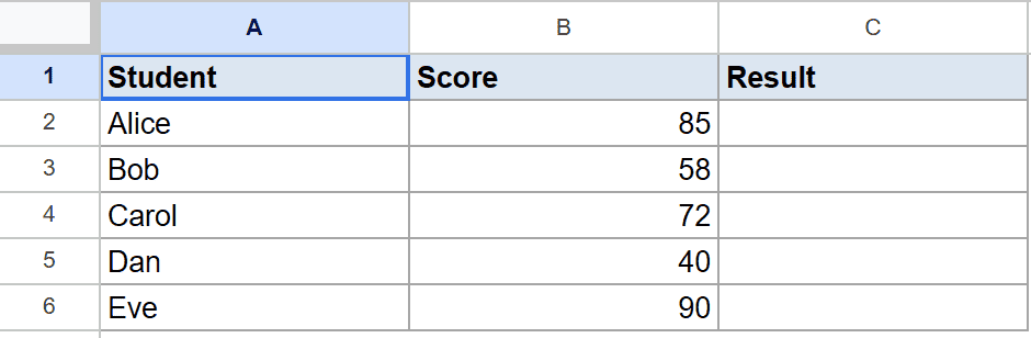
I want to mark each score as Pass when it is 60 or higher, and Fail otherwise.
Here is the formula:
=IF(B2>=60, "Pass", "Fail")
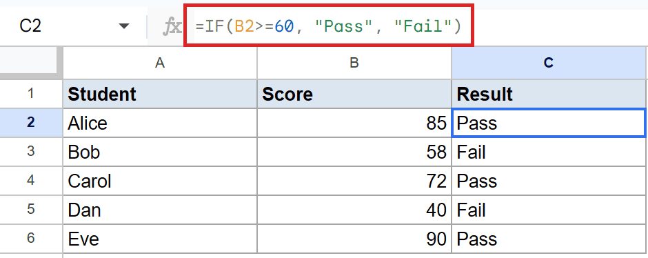
The test B2>=60 checks the score. When it is true the cell shows Pass, and when it is false it shows Fail.
Copy the formula down column C and every student gets a label. Alice, Carol, and Eve clear the bar, while Bob and Dan come up short.
Pro Tip: Instead of filling the formula down row by row, you can wrap it in ARRAYFORMULA to apply IF across the whole column in one cell, like =ARRAYFORMULA(IF(B2:B6>=60, “Pass”, “Fail”)). Same result, one formula.
Example 2: Calculate a Value Only When a Test Passes
The true and false parts do not have to be text. They can be calculations.
Below is the dataset with Customer in column A and Order amount in column B, across rows 2 to 6. Column C will hold the discount.
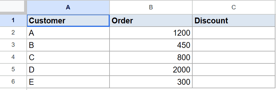
I want a ten percent discount on orders above 1000, and nothing on smaller orders.
Here is the formula:
=IF(B2>1000, B2*0.1, 0)
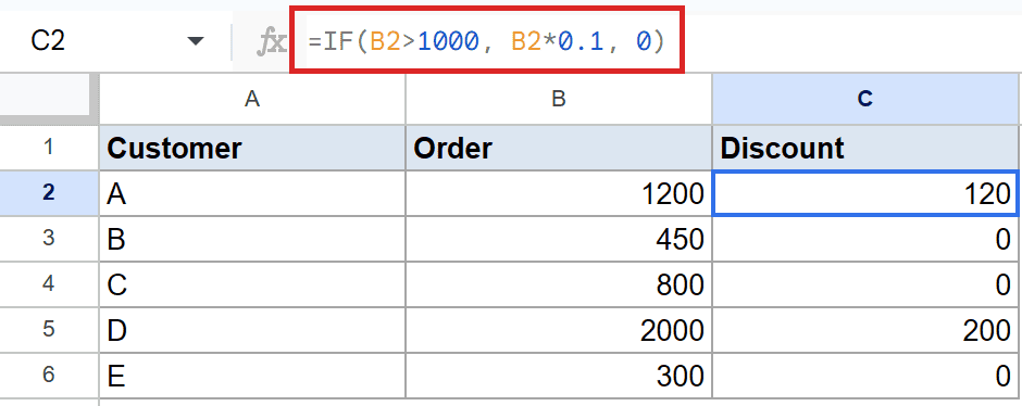
When the order clears 1000, the formula works out ten percent of the order. Otherwise it returns zero.
Customer A has an order of 1200, so the discount returns 120. Customer D, on a 2000 order, gets a discount of 200. The rest fall under the threshold and show zero.
Example 3: Assign Grades With Nested IF
When you need more than two outcomes, you can put an IF inside another IF.
Below is the dataset with Name in column A and Marks in column B, across rows 2 to 6. Column C is for the grade.
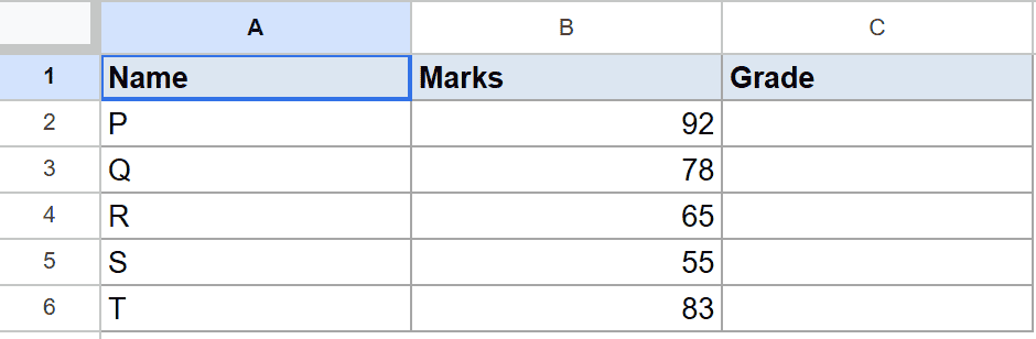
I want to sort marks into four bands, A, B, C, or D.
Here is the formula:
=IF(B2>=90, "A", IF(B2>=75, "B", IF(B2>=60, "C", "D")))
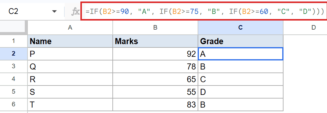
How this formula works:
- It checks the highest band first. If marks are 90 or more, it returns A and stops.
- If not, the next IF checks for 75 or more and returns B.
- The third IF checks for 60 or more and returns C.
- If none of the tests pass, the final value D is returned.
Order matters here. Each test only runs when the ones before it were false, so you go from the top band down.
Pro Tip: Deeply nested IFs get hard to read fast. For three or more bands, the IFS function is a cleaner alternative that lists each test and result in a flat sequence with no closing-bracket pileup at the end.
Example 4: Check Two Conditions With AND
A single IF tests one thing. Pair it with AND and you can require several things at once.
Below is the dataset with Employee in column A, Sales in column B, and Years of tenure in column C, across rows 2 to 5. Column D holds the bonus flag.
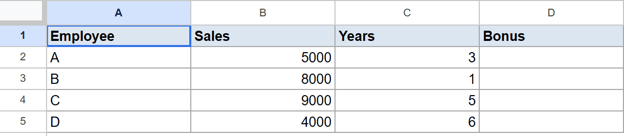
I want a Yes only when sales are at least 6000 and tenure is at least 2 years.
Here is the formula:
=IF(AND(B2>=6000, C2>=2), "Yes", "No")
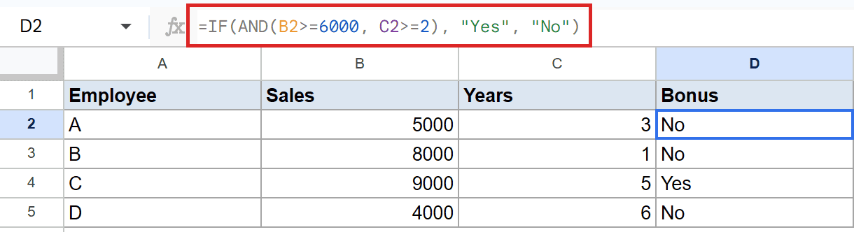
How this formula works:
- AND returns true only when both of its tests are true.
- The IF then shows Yes on a true result and No on a false one.
- Employee C is the only one who clears both bars, so only that row shows Yes.
Swap AND for OR if you want a Yes when either condition is met, rather than both.
Example 5: Handle Empty Cells Gracefully
IF is great for replacing blanks with a clear label so your sheet does not look broken.
Below is the dataset with Task in column A and Status in column B, across rows 2 to 5. One status cell is empty. Column C is the display.
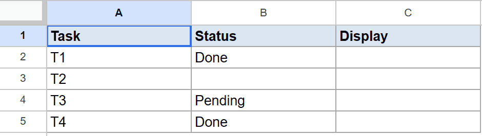
I want to show the status when it exists, and a clear note when the cell is blank.
Here is the formula:
=IF(B2="", "No status given", B2)
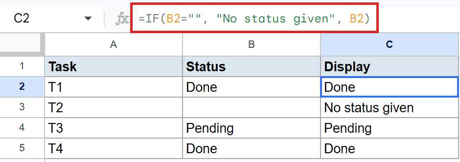
The test B2="" checks whether the status cell is empty. When it is, the formula shows the note. When it is not, it just shows the status.
So the filled rows display Done or Pending, while the empty row shows No status given instead of an awkward blank.
Tips & Common Mistakes
- Put text results in quotes. Words like “Pass” or “Yes” must sit inside double quotes. Numbers and cell references do not need them.
- Match your brackets. Nested IFs need one closing bracket for each IF you open. A missing bracket is the most common error. For many bands, consider IFS instead.
- Mind the comparison operator. Use
>=for “at least” and>for “more than”. Mixing them up is an easy way to get an off-by-one result at the boundary.
The IF function is the backbone of decision logic in a spreadsheet. Once you are comfortable with the true-and-false pattern, nesting and combining it with AND or OR follows naturally.
Try the formulas on your own data and tweak the tests to fit.
List of All Google Sheets Functions
Related Google Sheets Functions / Articles: