IFNA Function in Google Sheets

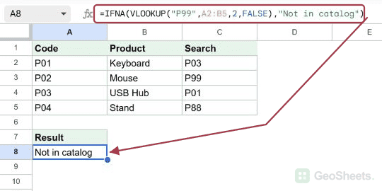
If you want to catch the #N/A error from a lookup and show a friendly message instead, the IFNA function in Google Sheets is what you need.

It runs your formula, and if the result comes back as #N/A, it swaps in whatever fallback you choose. In this article, I’ll show you how to use IFNA with VLOOKUP, MATCH, XLOOKUP, ARRAYFORMULA, and nested fallbacks.

IFNA Function Syntax in Google Sheets

Here is how the IFNA function is written:

=IFNA(value, value_if_na)

• value is the formula or expression you want to evaluate.
• valueifna is what to return if value comes back as #N/A. Any other error type passes through untouched.

IFNA is narrower than IFERROR on purpose. It reacts only to #N/A, so genuine bugs like #REF!, #DIV/0!, #NAME?, and #VALUE! still show up and you can fix them. If you want to swallow every error type, use IFERROR instead.

When to Use IFNA Function

• Replace #N/A from a failed VLOOKUP with a clean label like “Not found”.
• Catch missing matches from MATCH or XLOOKUP without hiding other formula errors.
• Cover an entire column of lookups in one cell using ARRAYFORMULA.
• Chain two lookups so a missing match in the first table falls through to a backup table.
• Keep real errors visible while still hiding the noisy #N/A cells.

Example 1: Replace Missing VLOOKUP Results With A Message

Let’s start with the classic case, wrapping IFNA around a VLOOKUP.

Below is the dataset, with a product code in column A, a product name in column B, and the codes to search in column C, across rows 2 to 6. Two of the search codes aren’t in the catalog.

You want to look up each search code and return its product name, with “Not in catalog” wherever the code is missing.

Here is the formula:

=IFNA(VLOOKUP(C2, A:B, 2, FALSE), "Not in catalog")

When the VLOOKUP finds a match, IFNA lets the product name through. The first row pulls back USB Hub for SKU03.

When the search code isn’t there, VLOOKUP would throw #N/A. IFNA catches it and the cell shows Not in catalog instead.

Pro Tip: IFNA only reacts to #N/A. If your VLOOKUP has a typo in the column index or a broken range, you’ll see #REF! or #VALUE! come through untouched. That’s by design, so you can spot real problems while still hiding clean misses.

Example 2: Tag Unknown Names From A MATCH Lookup

MATCH is another function that hits #N/A when a value isn’t in the search range, and IFNA wraps around it the same way.

Below is the dataset, with an employee name in column A and a search name in column B, across rows 2 to 6. A couple of the search names aren’t on the roster.

You want each search name’s row position in the roster, with “Not on roster” for the ones that don’t match.

Here is the formula:

=IFNA(MATCH(B2, $A$2:$A$6, 0), "Not on roster")

For names that exist in the roster, MATCH passes its position through. Olivia Brown is the fourth name in the range, so MATCH gives back 4.

For names that aren’t there, MATCH would error out. IFNA steps in and the cell shows Not on roster.

Example 3: Wrap XLOOKUP Calls Without A Built-In Default

XLOOKUP already accepts an if_not_found argument, but a lot of people skip it. IFNA gives you the same safety net from the outside.

Below is the dataset, with a sales rep in column A, their region in column B, and search reps in column C, across rows 2 to 6. Two of the search reps aren’t in the list.

You want each search rep’s region, with “Unknown rep” anywhere the name doesn’t appear.

Here is the formula:

=IFNA(XLOOKUP(C2, $A$2:$A$6, $B$2:$B$6), "Unknown rep")

XLOOKUP scans column A for the search rep and pulls the matching region from column B. When it finds the rep, the region passes through.

When the rep is missing, XLOOKUP would normally throw #N/A. IFNA catches that and writes Unknown rep into the cell.

Pro Tip: XLOOKUP’s fourth argument does the same job as IFNA. =XLOOKUP(C2, A:A, B:B, “Unknown rep”) is shorter. Use IFNA when you already wrote the lookup and just want to bolt on a fallback without rewriting.

Example 4: Use ARRAYFORMULA To Fall Back Over A Whole Column

If you’d rather write one formula for the entire column instead of filling down, wrap the IFNA call in ARRAYFORMULA.

Below is the dataset, with a city in column A, its tax rate in column B, and search cities in column C, across rows 2 to 6. A couple of the search cities aren’t listed.

You want one formula in D2 that fills the whole D column with the matching tax rate, and shows “Rate unknown” for missing cities.

Here is the formula:

=ARRAYFORMULA(IFNA(VLOOKUP(C2:C6, A2:B6, 2, FALSE), "Rate unknown"))

How this formula works:

• ARRAYFORMULA tells Google Sheets to run the inner formula across the entire C2:C6 range, not just one cell.
• VLOOKUP runs once per row inside the array, looking up each search city in A2:B6.
• IFNA wraps each row’s result. Matching cities show their tax rate. Missing ones show Rate unknown.

The array spills down from D2 with all five answers in one shot. If a new row gets added to the search list, just extend the range and the fallback applies automatically.

Example 5: Chain Two Lookups Before Falling Back To Text

Here’s a pattern that surprises people. You can nest IFNA inside another IFNA to try a second table when the first one comes up empty.

Below is the dataset, with a primary code and region in columns A and B, a backup code and region in columns C and D, and codes to search in column E, across rows 2 to 6.

You want each search code’s region from the primary table, with a fall-through to the backup table, and “Region unknown” only when both tables fail.

Here is the formula:

=IFNA(VLOOKUP(E2, A:B, 2, FALSE), IFNA(VLOOKUP(E2, C:D, 2, FALSE), "Region unknown"))

How this formula works:

• The outer IFNA runs the first VLOOKUP against columns A and B.
• If that lookup finds a match, the matching region passes through.
• If the first VLOOKUP comes back #N/A, the outer IFNA kicks off the second VLOOKUP against columns C and D.
• If the backup lookup also fails, the inner IFNA writes Region unknown.

So a code that lives only in the backup table still resolves, while a code in neither table lands on the final text fallback.

Pro Tip: Order matters when you nest IFNA. The outer call is your first lookup, the inner call is your fallback. Flip them and you’re searching the backup table first, which is rarely what you want.

Tips & Common Mistakes

• IFNA only catches #N/A. It will not hide #REF!, #DIV/0!, #NAME?, or #VALUE!. That’s a feature, not a bug. If you want to mask every error type, reach for IFERROR instead.
• Don’t wrap the lookup value, wrap the whole call. Putting IFNA around just C2 won’t catch anything. The #N/A comes from the VLOOKUP or MATCH, so IFNA has to sit around the full lookup expression.
• Watch for an exact-match flag on VLOOKUP. If you forget the FALSE (or 0) on the fourth argument, VLOOKUP does an approximate match and may return the wrong row instead of #N/A. IFNA won’t save you from that, because the lookup isn’t returning an error in the first place.

IFNA is the cleanest way to handle missing lookup matches without silencing every other error in your sheet. Wrap the lookup, supply a fallback string or value, and your sheet stays readable.

Start with a plain label like “Not found” or “Unknown”, and reach for nested IFNA only when you genuinely have a second source to try.

List of All Google Sheets Functions

Related Google Sheets Functions / Articles:

• ISNA Function in Google Sheets
• XLOOKUP Function in Google Sheets
• VLOOKUP Function in Google Sheets
• LOOKUP Function in Google Sheets
• IFS Function in Google Sheets