
To freeze the top row in Google Sheets, choose View > Freeze > 1 row. The header stays visible while the rows below it scroll.
You can also freeze several leading rows, drag the freeze divider, or return to View > Freeze > No rows to unfreeze them.
Freeze the top row in Google Sheets
- Open the sheet that has your header row.
- Choose View > Freeze > 1 row.
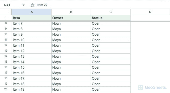
- Scroll down and confirm that row 1 remains above the freeze divider.
In our Windows Chrome test, row 1 stayed visible while cell A30 was selected. A gray divider separated the frozen header from the scrolling rows.
Freeze two or more rows
Use this method when a heading spans several rows.
- Select a cell in the last row that should remain visible.
- Choose View > Freeze.
- Select Up to row 3, or the current row number shown in your menu.
We selected A3 and chose Up to row 3. Sheets pinned rows 1 through 3 together.
Freeze rows with the drag handle
A thicker gray divider appears near the top-left corner of the grid. Drag its horizontal section down to the boundary below the last row you want frozen.
In the test sheet, dragging the divider from the row 3 boundary back to the row 1 boundary changed the sheet from three frozen rows to one.
Unfreeze rows
Choose View > Freeze > No rows. The divider returns to the top edge and every row scrolls normally.
Is there a freeze-row keyboard shortcut?
Google’s Sheets shortcut list does not include a dedicated freeze-row command. Use the View menu or the draggable divider.
Google’s freeze rows and columns instructions document the View menu and No rows option.
If you print a long sheet, Google can repeat frozen rows on each page. Open Print, expand Headers & footers, then select Repeat frozen rows.
Other Google Sheets articles you may also like