
To freeze the first column in Google Sheets, choose View > Freeze > 1 column. Column A stays visible while the rest of the sheet scrolls horizontally.
Use Up to column for several identifying columns, or drag the vertical freeze divider to the column boundary you need.
Freeze the first column in Google Sheets
- Open a sheet with labels in column A.
- Choose View > Freeze > 1 column.
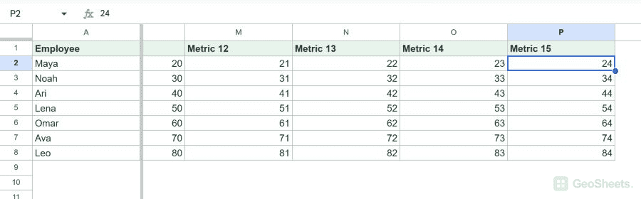
- Scroll right and confirm that column A remains beside the visible data.
Our Windows Chrome test pinned column A. After scrolling right, column A remained visible beside columns J through P.
Freeze two or more columns
- Select a cell in the last column that should remain visible.
- Choose View > Freeze.
- Select Up to column C, or the current column letter shown in your menu.
We selected C1 and chose Up to column C. Columns A through C stayed pinned while column P was visible.
Freeze columns with the drag handle
At the top-left of the grid, drag the thicker vertical divider to the right. Drop it after the last column you want frozen.
In our test, dragging the divider from the column C boundary back to the column A boundary changed three frozen columns to one.
Unfreeze columns
Choose View > Freeze > No columns. The divider returns to the left edge and all columns scroll normally.
Is there a freeze-column keyboard shortcut?
Google’s Sheets shortcut list does not include a dedicated freeze-column command. Use the View menu or the draggable divider.
You can freeze rows and columns in the same sheet. This keeps a header row and identifying columns visible while you scroll in either direction.
For printouts, Google documents a separate Repeat frozen columns setting under Print > Headers & footers.
Other Google Sheets articles you may also like