
Select a cell in the column you want to hide, then press Ctrl + Alt + 0 on Windows. The column disappears from view while its values and formulas remain available.
Hide column keyboard shortcut
Windows: Ctrl + Alt + 0
Mac: Command + Option + 0
Use the number-row zero. You can select a cell in the column or click its letter. In our Windows test, selecting C2 was sufficient to hide column C.
Hide a helper column without deleting it
- Select C2, or click the C column heading.
- Press the shortcut for your computer.
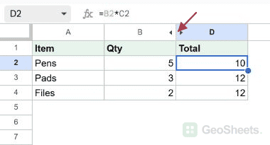
- Check that the column headings now jump from B to D.
Our example stores quantities in B, prices in C, and totals in D. After hiding C, the formula =B2*C2 still returns 10. The other totals remain 12 and 12.
Hide columns using the mouse
- Click a column letter. To hide adjacent columns, drag across their letters.
- Right-click a selected column heading.
- Choose Hide column, or the command naming the selected columns.
Use this route if a keyboard layout, browser, or operating-system shortcut prevents the key combination from reaching Sheets. The menu label reflects your selection.
Show the hidden columns again
Click the small arrow at the gap in the column headings. You can also select columns on both sides, right-click their headings, and choose Unhide columns.
For hidden C, select B through D. The keyboard alternative is Ctrl + Shift + 0 on Windows or Command + Shift + 0 on Mac.
Choose hiding, grouping, or freezing
Hide a column when you want it out of the working view. Group columns when you want a visible control for repeatedly collapsing and expanding related fields.
Freeze a column when you want it to stay visible while scrolling. These actions serve different purposes and do not replace deleting data.
Before printing, inspect the print preview. If the hidden information belongs in the printed report, unhide those columns first.
Other Google Sheets articles you may also like