
To unhide columns in Google Sheets, select the headings on either side of the gap, then use the shortcut below. The hidden data reappears in its original position.
Unhide column keyboard shortcut
Windows: Ctrl + Shift + 0
Mac: Command + Shift + 0
Select a range spanning the hidden column before pressing the shortcut. Use the 0 key above the letters. Keyboard layouts or system shortcuts can interfere.
Restore column C step by step
- Click the column letter B.
- Hold Shift and click D to select across the hidden gap.
- Press the shortcut for your computer.
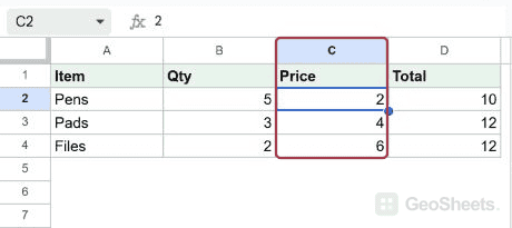
- Check that column C reappears between B and D.
For this example, you can also enter B:D in the Name box and press Enter to select the required range.
The example restores the Price column. The existing totals remain 10, 12, and 12.
Use the arrows or right-click menu
Look for the small arrows between the column letters around the gap. Click an arrow to show the hidden columns there.
Alternatively, select across the gap, right-click a selected column heading, and choose Unhide columns. This is useful when the keyboard shortcut is intercepted.
Unhide every column in the sheet
- Click the blank square where the row numbers meet the column letters, at the top-left of the grid.
- Press the unhide column shortcut.
Selecting the whole sheet also handles a hidden column A, where there is no visible heading before the gap.
When missing columns have another cause
A collapsed group uses a + control. Expand the group when you want to restore its contents while keeping the grouping structure.
Filters hide rows according to conditions. They do not create “filter-hidden columns.” A missing column letter indicates a different cause, such as manual hiding.
Freezing keeps columns visible while scrolling; it does not delete or hide their contents. Hiding and unhiding also leave stored values and ordinary cell references intact.
Other Google Sheets articles you may also like