
Select a cell in the row and press Ctrl + Alt + 9 to hide that row in Google Sheets. The row’s data stays in the spreadsheet.
Hide one or several rows
Our test selected B3 and hid row 3, so selecting the full row first is not required. For several adjacent rows, select their row numbers before using the shortcut.
- Select a cell in the row, or select the relevant row numbers.
- Press Ctrl + Alt + 9 on Windows. On Mac, use Command + Option + 9.
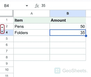
- Check that the row numbers skip the hidden rows.
Use the right-click menu
Right-click the selected row numbers and choose Hide row or Hide rows. The command label includes the selected range when more than one row is involved.
Show hidden rows again
Click the small arrows between the surrounding row numbers. You can also select the neighboring rows, right-click, and choose the option to unhide the intervening rows.
Understand what hiding changes
Hiding is a display change. Ordinary SUM formulas can still include the hidden values, and collaborators with access may unhide them. It does not protect confidential data.
Distinguish hidden, filtered and grouped rows
A filter hides rows that fail its conditions. A collapsed group hides related rows behind a group control. Use the relevant filter or plus button when those features caused the disappearance.
Other Google Sheets articles you may also like