
If you want to swap a specific piece of text inside a cell for something else, the SUBSTITUTE function in Google Sheets is what you need.
It scans the cell, finds every match of the old text, and replaces it with the new text you choose. In this article, I’ll show you how to use SUBSTITUTE to update phone numbers, swap words in sentences, strip prefixes, target a single occurrence, and clean multiple tokens at once.
SUBSTITUTE Function Syntax in Google Sheets
Here is how the SUBSTITUTE function is written:
=SUBSTITUTE(text_to_search, search_for, replace_with, [occurrence_number])
- text_to_search is the text or cell reference you want to edit.
- search_for is the piece of text you want to replace.
- replace_with is the new text that takes its place. Passing
""(empty string) deletes the matched text. - occurrence_number is optional. Without it, every match gets replaced. Pass
1,2, etc. to target only that specific match.
SUBSTITUTE works by matching the actual text content. If you need to replace something at a fixed position, like the third through fifth characters of a code, look at REPLACE instead.
When to Use SUBSTITUTE Function
- Update an area code, country code, or any fixed token inside a column of phone numbers or IDs.
- Swap a word or short phrase across an entire column of sentences.
- Strip a known prefix or suffix from product codes by passing
""as the replacement. - Replace only a specific occurrence (like the second comma) without touching the others.
- Clean up multiple shorthand tokens in one pass by nesting SUBSTITUTE inside SUBSTITUTE.
Example 1: Replace An Area Code In Phone Numbers
Let’s start with the classic case, swapping one piece of text for another inside a column of phone numbers.
Below is the dataset, with phone numbers in column A, across rows 2 to 6. Every number has the same middle three digits that we want to swap.
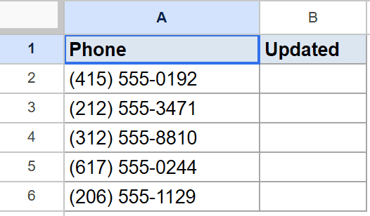
You want a new column that replaces the middle three digits in each phone number with a fresh value.
Here is the formula:
=SUBSTITUTE(A2, "555", "844")
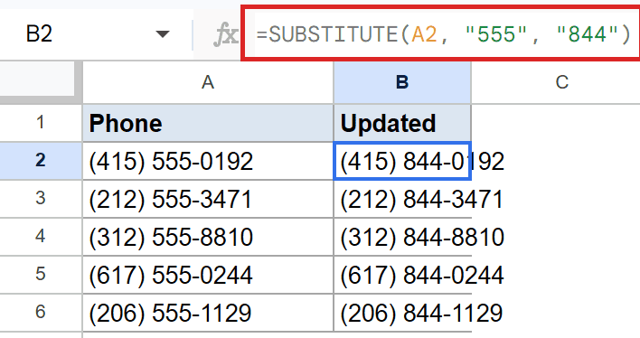
SUBSTITUTE scans the cell for the text in the second argument, then writes the third argument in its place. The first row becomes (415) 844-0192. Every other row follows the same pattern.
Since SUBSTITUTE acts on content, it finds the digits no matter where they sit inside the string. If a row had a different layout, like an international format, the same formula would still work.
Pro Tip: SUBSTITUTE is case-sensitive. “555” matches only “555”, and “abc” will not match “ABC”. If you need case-insensitive replacement, look at REGEXREPLACE, which lets you pass a regex flag for case folding.
Example 2: Swap A Word Inside A Sentence
SUBSTITUTE happily replaces whole words inside longer sentences, which is handy for rewording status updates or report lines.
Below is the dataset, with a status line in column A, across rows 2 to 6. Each line uses the same verb that we want to rewrite.
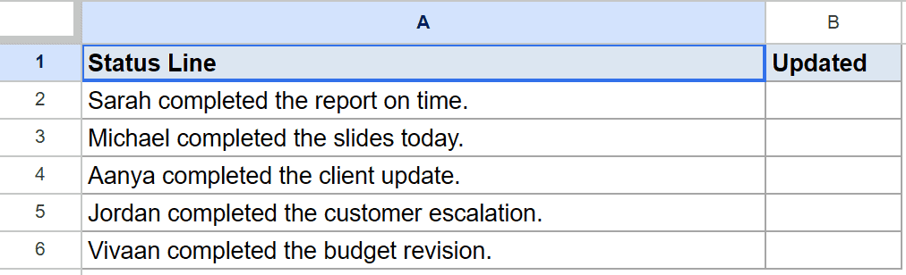
You want every “completed” replaced with “finalized”, leaving the rest of the sentence alone.
Here is the formula:
=SUBSTITUTE(A2, "completed", "finalized")
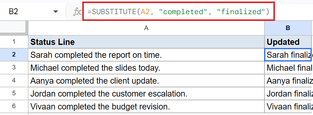
SUBSTITUTE finds the word inside each sentence and swaps it. The first row becomes Sarah finalized the report on time. The other rows update the same way.
The surrounding text doesn’t change at all. SUBSTITUTE touches only the matched substring, so names, dates, and other details stay intact.
Example 3: Strip A Prefix From Product Codes
If you pass an empty string as the replacement, SUBSTITUTE removes the matched text instead of replacing it. That’s a clean way to strip a known prefix or suffix.
Below is the dataset, with raw product codes in column A, across rows 2 to 6. Every code starts with the same prefix that we want to remove.
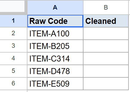
You want a cleaned column that has the same codes minus the prefix.
Here is the formula:
=SUBSTITUTE(A2, "ITEM-", "")
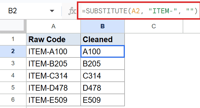
The empty quotes "" tell SUBSTITUTE to replace the matched text with nothing. The first row becomes A100, the second becomes B205, and the rest of the column follows suit.
This trick is useful for removing repeated characters too. For example, =SUBSTITUTE(A2, " ", "") strips every space out of a cell.
Pro Tip: Pair LEN with SUBSTITUTE to count how often a character appears in a string. The expression LEN(A2) minus LEN(SUBSTITUTE(A2, ” “, “”)) gives you the count of spaces in A2, which is also the classic word-count workaround in Google Sheets. See the LEN function article for the full pattern.
Example 4: Target Only The Second Match To Replace
By default SUBSTITUTE swaps every match. Pass an occurrence number as the fourth argument and it touches only that one match.
Below is the dataset, with a comma-separated list in column A, across rows 2 to 6. We want to highlight only the boundary between the second and third items.
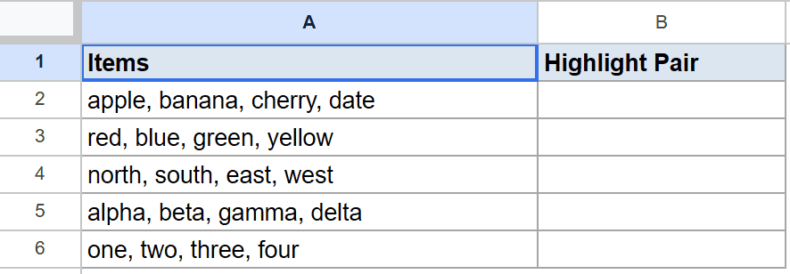
You want the second comma in each row replaced with a pipe separator, leaving the other commas alone.
Here is the formula:
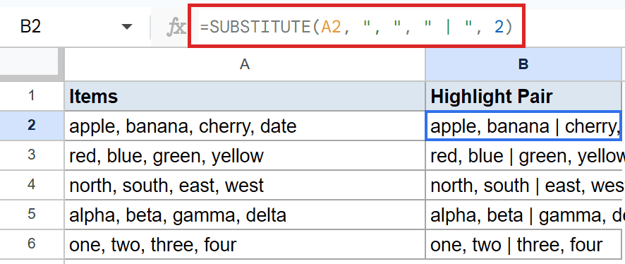
=SUBSTITUTE(A2, ", ", " | ", 2)
How this formula works:
- The first three arguments work the same as before. SUBSTITUTE looks for
", "and the planned replacement is" | ". - The fourth argument tells SUBSTITUTE to act only on the second occurrence of the search text.
- Every other match stays untouched.
The first row becomes apple, banana | cherry, date. The other rows follow the same shape, with the pipe sitting where the second comma used to be.
Pro Tip: The occurrence number must be a positive whole number. Pass zero or a negative value and SUBSTITUTE returns #VALUE!. If the cell has fewer matches than the number you pass, SUBSTITUTE leaves the cell unchanged.
Example 5: Clean Two Different Abbreviations At Once
When you need to replace more than one thing in a single cell, nest one SUBSTITUTE inside another. Each layer handles its own swap.
Below is the dataset, with mailing addresses in column A, across rows 2 to 6. Some rows abbreviate “Street” as “St.” and others use “Ave.” for “Avenue”.
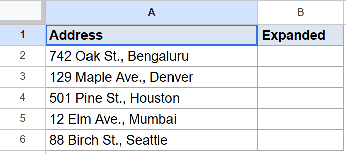
You want both abbreviations expanded into the full words in one shot.
Here is the formula:
=SUBSTITUTE(SUBSTITUTE(A2, "St.", "Street"), "Ave.", "Avenue")
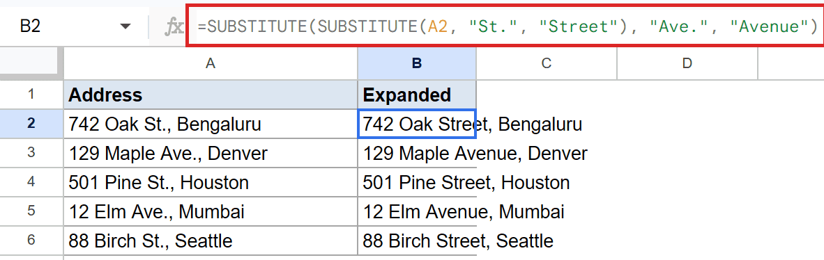
How this formula works:
- The inner SUBSTITUTE runs first. It replaces
St.withStreetinside the cell. - The outer SUBSTITUTE takes that updated string as its input and replaces
Ave.withAvenue. - Both swaps land in the same output cell.
So the first row becomes 742 Oak Street, Bengaluru, and rows that had Ave. come back with the full Avenue. Nest a third SUBSTITUTE if you need to clean a third token.
Tips & Common Mistakes
- SUBSTITUTE is case-sensitive. A search for “completed” will not match “Completed” or “COMPLETED”. If you need case-insensitive replacement, switch to REGEXREPLACE with a case-fold flag, or normalize the column with UPPER or LOWER first.
- Pass
""to delete, not a space. Putting a single space inside the quotes leaves a stray space behind. To strip a token completely, use the empty string"". To collapse “ITEM-” into something readable, that’s exactly what you want. - Don’t confuse SUBSTITUTE with REPLACE. SUBSTITUTE finds text by content and swaps every match (or one specific occurrence). REPLACE works by position, replacing a fixed range of characters regardless of what they are. Use SUBSTITUTE when you know the text. Use REPLACE when you know the position.
SUBSTITUTE is the go-to function for content-based text cleanup in Google Sheets. Point it at the text, give it the search-and-replace pair, and the whole column gets rewritten.
Add an occurrence number when you need to target a single match, pass an empty string when you want to delete, and nest the calls when you have more than one swap to make.
List of All Google Sheets Functions
Related Google Sheets Functions / Articles: