
If you want to grab the largest number from a list, but only from the rows that match one or more conditions, the MAXIFS function in Google Sheets does it in a single call. You hand it the values to look through, a range with the labels to check, and what those labels need to match.
In this article, I’ll walk through five practical MAXIFS setups. You’ll see it with a single text criterion, a numeric comparison, two-criteria combos, date ranges, and a mixed text-plus-number filter.
MAXIFS Function Syntax in Google Sheets
The MAXIFS function returns the largest value from a range, restricted to rows that meet every criterion you pass.
=MAXIFS(range, criteria_range1, criterion1, [criteria_range2, criterion2], ...)
- range is the column of numbers you want the maximum from.
- criteria_range1 is the column where the first condition is checked.
- criterion1 is the value that criteria_range1 must match. Text and operators go in double quotes.
- criteria_range2, criterion2, … are optional extra pairs. Add as many as you need.
All ranges must be the same height. If the value range spans six rows, every criteria range must span six rows too, or MAXIFS throws an error.
When to Use MAXIFS Function
- Pull the highest figure for one category from a longer table (top sales in the East region, top score in Math).
- Find the largest value above or below a threshold without sorting the data.
- Combine two or more filters in one shot (one student, one subject) without a helper column.
- Get the biggest order placed inside a date window.
- Stack a text label and a number rule together to peel one max value out of a mixed dataset.
Example 1: Maximum Sales for One Region
Let’s start with the most common MAXIFS pattern, one text criterion.
Below is the dataset. Column A has the rep, column B has the region, and column C has the sales figure.
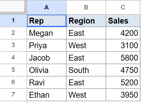
I want the largest sales figure across all rows where the region is East.
Here is the formula:
=MAXIFS(C2:C7, B2:B7, "East")
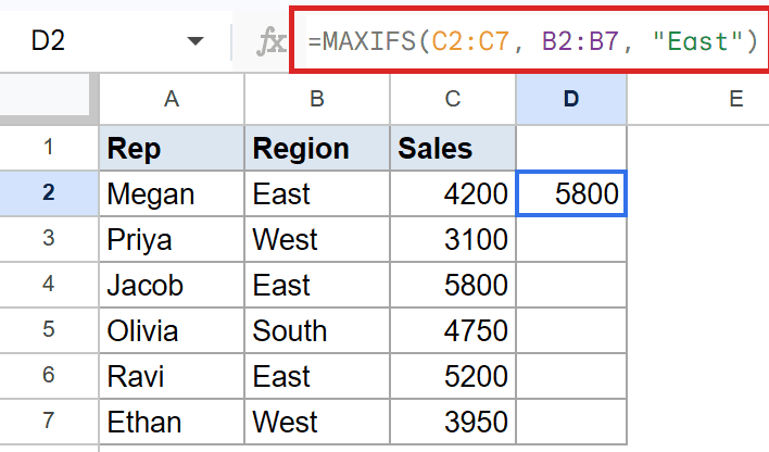
MAXIFS walks column C and only considers the rows where column B says East. There are three East rows (Megan at 4200, Jacob at 5800, and Ravi at 5200), and the biggest of those is 5800.
The other rows (West, South) are ignored. Notice the criterion is wrapped in double quotes since it’s text.
Pro Tip: If you want the total sales for East instead of the max, swap MAXIFS for SUMIFS. Same argument order, different math.
Example 2: Largest Revenue Where Units Beat a Threshold
The criterion does not have to be text. You can also pass a numeric comparison.
Below is the dataset. Column A has the product, column B has units sold, and column C has revenue.
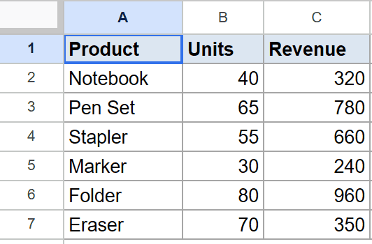
I want the largest revenue from rows where units sold are over 50.
Here is the formula:
=MAXIFS(C2:C7, B2:B7, ">50")
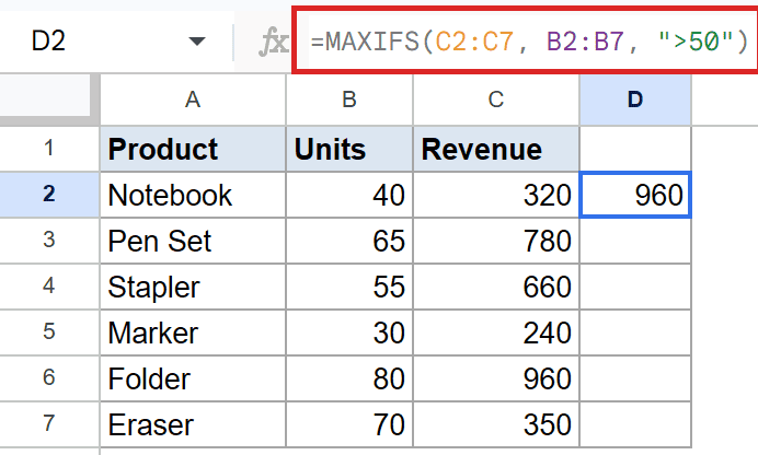
The comparison ">50" keeps only rows where the unit count is greater than 50. Pen Set (65 units, 780), Stapler (55 units, 660), Folder (80 units, 960), and Eraser (70 units, 350) all qualify. The biggest revenue among those is 960.
The whole comparison (the operator and the number) sits inside one pair of double quotes. That quoting trips up a lot of first-time users.
Example 3: Top Score for One Student in One Subject
MAXIFS shines when you have more than one filter to apply.
Below is the dataset. Column A has the student, column B has the subject, and column C has the score.
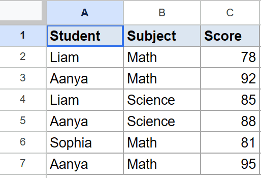
I want the highest score for Aanya in Math specifically.
Here is the formula:
=MAXIFS(C2:C7, A2:A7, "Aanya", B2:B7, "Math")
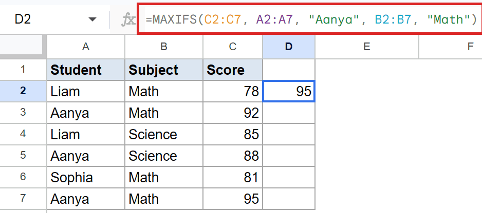
Two criteria pairs are applied. Column A must equal Aanya AND column B must equal Math. Aanya has two Math rows (92 and 95) and one Science row (88). The Science row is filtered out. Between 92 and 95, the result is 95.
Both criteria need to be true at the same time. A row is only included if every criteria range matches its corresponding criterion.
Example 4: Highest Order Inside a Date Range
Dates work fine as criteria. You just have to build the comparison with the DATE function so Sheets reads it as a date.
Below is the dataset. Column A has the order ID, column B has the order date, and column C has the amount.
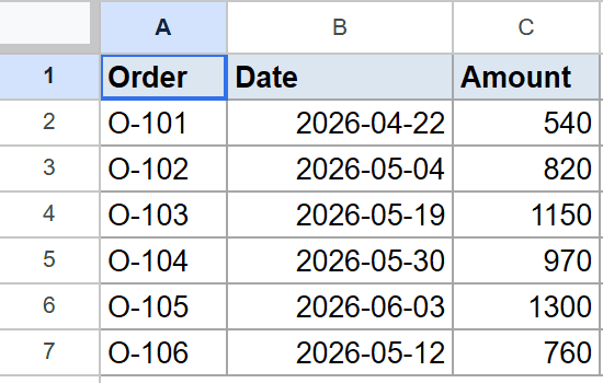
I want the biggest order placed in May 2026 (between May 1 and May 31 inclusive).
Here is the formula:
=MAXIFS(C2:C7, B2:B7, ">="&DATE(2026,5,1), B2:B7, "<="&DATE(2026,5,31))
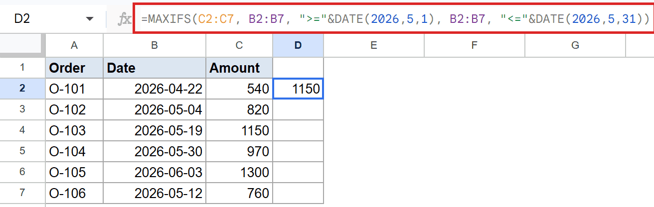
The criteria use the same column twice, once for the lower bound and once for the upper bound. Three orders fall inside May 2026 (O-102 at 820, O-103 at 1150, O-104 at 970, O-106 at 760). The biggest of those is 1150.
The & operator glues the comparison operator to the DATE result. Without DATE, Sheets would treat "2026-05-01" as plain text and the comparison would not match real dates.
Pro Tip: You can use the same range twice as I did here, or two different ranges. MAXIFS doesn’t care if criteria ranges repeat, as long as each pair lines up correctly.
Example 5: Top Bonus for a Department With a Tenure Floor
Mixing a text filter with a numeric threshold is a common real-world setup.
Below is the dataset. Column A has the employee, column B has the department, column C has tenure in years, and column D has the bonus.
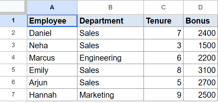
I want the largest bonus paid to Sales staff with five or more years of tenure.
Here is the formula:
=MAXIFS(D2:D7, B2:B7, "Sales", C2:C7, ">=5")
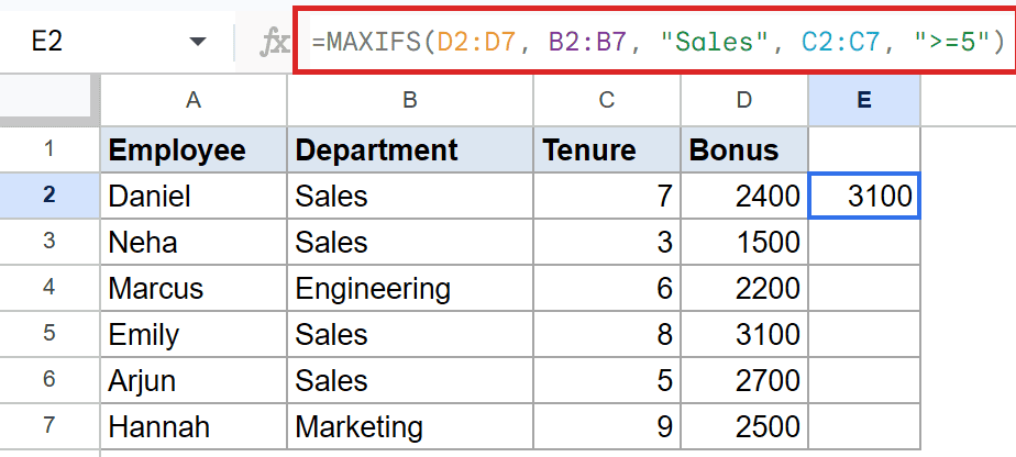
Two filters narrow the rows. Sales staff with tenure of 5 or more includes Daniel (7 years, 2400), Emily (8 years, 3100), and Arjun (5 years, 2700). Neha is excluded (3 years, under the cutoff). The biggest bonus across those three is 3100.
Notice that Marcus has 6 years but he’s in Engineering, so he doesn’t qualify either. Both conditions need to be true.
Tips & Common Mistakes
- Match the range sizes. Every range you pass (the value range and each criteria range) must be exactly the same height. Mixing C2:C7 with B2:B10 throws
#N/Aor#VALUE!. This is the most common MAXIFS mistake. - Quote operators and text. Conditions like
">=50","<>East", or"Aanya"all need double quotes. Numbers as exact matches (like5) don’t need quotes, but anything with>,<,>=,<=,<>does. - Empty result returns 0. If no rows match your criteria, MAXIFS returns 0, not an error. Don’t read that as a real maximum. If you need to spot the no-match case, wrap MAXIFS in an IF that checks for it.
MAXIFS is the cleanest way to pull a conditional maximum out of a Google Sheets table.
You’ve now seen it with a single text criterion, a numeric comparison, two-text filters, a date range, and a mixed text-plus-number setup. Pass it a value range and one or more criteria pairs, and you get the largest matching number back in one cell.
List of All Google Sheets Functions
Related Google Sheets Functions / Articles: