
If you have two or more ranges sitting side by side and you want to combine them into a single tall list, the VSTACK function in Google Sheets does it in one shot. You pass it the ranges, and it stacks them vertically into a spilled grid.
In this article, I’ll walk through five common VSTACK setups. You’ll see it stacking two ranges, three ranges, a literal header above a table, a raw list combined with a sorted one, and a vertical literal placed above a single column.
VSTACK Function Syntax in Google Sheets
The VSTACK function stacks two or more arrays on top of each other and spills the combined grid into the surrounding cells.
=VSTACK(range1, [range2, ...])
- range1 is the first array (cell range or literal array).
- range2, … are additional arrays to stack below the first. Add as many as you need.
Every range must have the same number of columns. VSTACK lines them up by column position, so a 2-column range stacked on a 3-column range throws an error. The result spills automatically, so the formula goes in one cell and the rest fills in.
When to Use VSTACK Function
- Combine two tables sitting side by side into one tall list.
- Append a fresh header row above an existing data range.
- Merge quarterly or monthly chunks into one rolling list.
- Stack a sorted list under a raw list (or vice versa) without losing the order.
- Build a custom header block on the fly, then stack the data below it.
Example 1: Stack Two Ranges of the Same Shape
Let’s start with the most common VSTACK pattern, two ranges side by side that you want stacked end to end.
Below is the dataset. Columns A and B hold the Q1 reps and their sales. Columns D and E hold the Q2 reps and their sales.
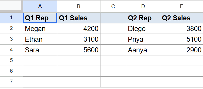
I want one tall list with the Q2 rows sitting underneath the Q1 rows.
Here is the formula:
=VSTACK(A2:B4, D2:E4)
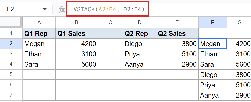
VSTACK takes the Q1 block (three rows, two columns) and puts the Q2 block (three rows, two columns) right under it. The output spills into six rows starting at the formula cell, two columns wide. Megan, Ethan, and Sara appear first, then Diego, Priya, and Aanya.
Both source ranges are the same width (two columns each), which is the one rule VSTACK enforces. If they didn’t match, the formula would error out instead of stacking.
Pro Tip: To stack ranges side by side instead of top to bottom, use HSTACK. Same syntax, horizontal layout. VSTACK is vertical, HSTACK is horizontal.
Example 2: Stack Three Quarterly Ranges Together
VSTACK doesn’t stop at two arguments. You can pass as many ranges as you need.
Below is the dataset. Three side-by-side blocks of two columns each, holding the Q1, Q2, and Q3 reps and their sales.
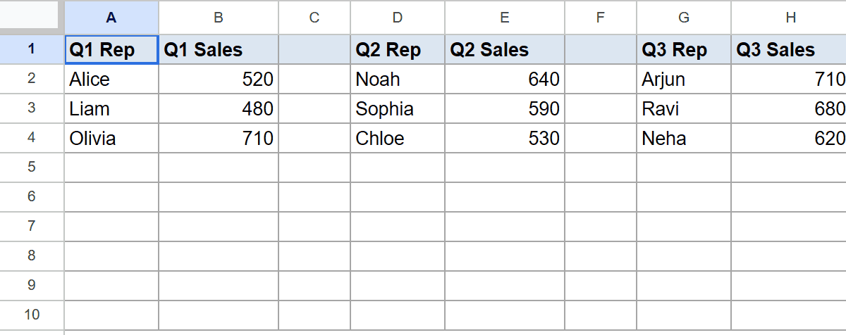
I want all three quarters merged into one tall list.
Here is the formula:
=VSTACK(A2:B4, D2:E4, G2:H4)
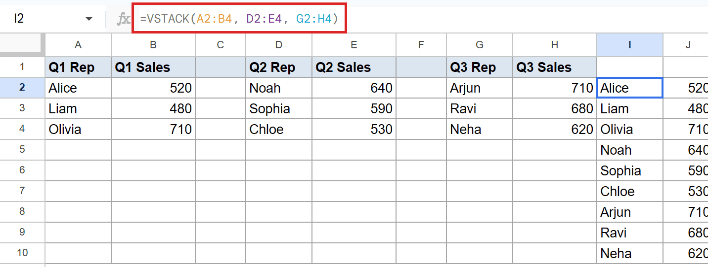
Each three-row block stacks under the one above it. The spill is nine rows tall and two columns wide. Q1 sits on top (Alice, Liam, Olivia), Q2 in the middle (Noah, Sophia, Chloe), and Q3 at the bottom (Arjun, Ravi, Neha).
You can keep adding ranges. A four-quarter rollup is the same formula with one more argument. As long as every range is two columns wide, VSTACK doesn’t care how many you pass.
Example 3: Add a Literal Heading Row on Top of Data
You can mix literal arrays with cell ranges. This is handy when you want a custom header sitting above a table.
Below is the dataset. Column A has employee names and column B has their final scores. There’s no header row in the data itself.
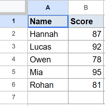
I want to glue a header row (Employee, Final Score) on top of the existing data.
Here is the formula:
=VSTACK({"Employee","Final Score"}, A2:B6)
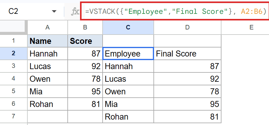
The {"Employee","Final Score"} is an inline literal array. It’s a single row with two columns. VSTACK stacks the five-row data range underneath it, so the spill is six rows total, two columns wide, with the header sitting on top.
Curly braces hold the literal array. Commas inside the braces separate columns in the same row.
Pro Tip: Inside `{}`, a comma means “next column” and a semicolon means “next row”. So `{“A”,”B”}` is one row with two columns, while `{“A”;”B”}` is two rows with one column.
Example 4: Stack a Raw List With a Sorted List
VSTACK arguments don’t have to be plain ranges. You can pass any array-returning expression, including SORT.
Below is the dataset. Columns A and B hold new hires in the order they joined. Columns D and E hold legacy employees in random order.
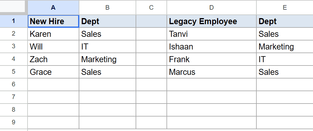
I want the new hires listed as-is on top, with the legacy employees sorted alphabetically below them.
Here is the formula:
=VSTACK(A2:B5, SORT(D2:E5))
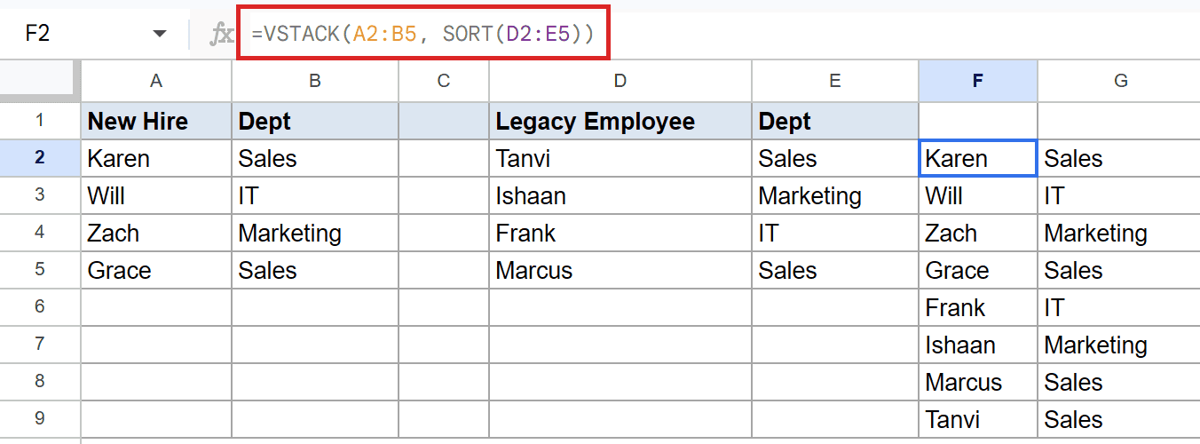
The first argument is the raw new-hire range. The second is SORT wrapped around the legacy range, which orders those rows alphabetically by the first column. VSTACK stacks the two arrays. New hires (Karen, Will, Zach, Grace) keep their original order on top, and the legacy block sorts to Frank, Ishaan, Marcus, Tanvi.
This is the real strength of VSTACK. Any argument can be a function call as long as it returns an array. Wrap your inputs in SORT, UNIQUE, FILTER, or even another VSTACK, and the whole thing stacks together.
Example 5: Stack a Vertical Literal Above a Single Column
Literal arrays can also be vertical, useful for stacking a multi-row header block on a single column.
Below is the dataset. Column A holds a list of cities with no header.
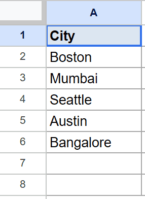
I want a two-row header (Top Cities, then a separator line) sitting on top of the city list.
Here is the formula:
=VSTACK({"Top Cities";"---"}, A2:A6)
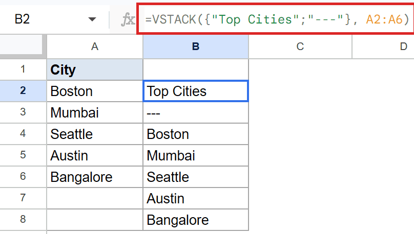
The semicolon inside {} makes the literal array vertical. {"Top Cities";"---"} is two rows tall and one column wide. VSTACK puts the five-city range underneath it, so the spill is seven rows tall and one column wide. Boston, Mumbai, Seattle, Austin, and Bangalore sit below the header block.
Notice both pieces are one column wide. If the city list had two columns, the literal header would also need to be two columns wide, or VSTACK would error.
Tips & Common Mistakes
- Match the column count, not the row count. Every range in VSTACK must have the same number of columns. Row counts can vary (a 3-row block under a 10-row block is fine). A 2-column range mixed with a 3-column range throws
#VALUE!. - Spill area must be empty. VSTACK spills into cells around the formula. If any of those cells already have content, you’ll see
#REF!with the message “Array result was not expanded because it would overwrite data”. Clear the spill area or move the formula. - Use literals for inline headers, not extra ranges. When you only need a header, type it inline with
{}instead of putting it in a helper range somewhere on the sheet. It keeps the formula self-contained and easier to maintain.
VSTACK is the cleanest way to glue multiple ranges into one tall list in Google Sheets.
You’ve now seen it stacking two and three ranges of the same shape, adding a horizontal header literal, mixing a SORT call as one of its arguments, and stacking a vertical literal block on top of a single column. Pick the ranges, line up the column counts, and the formula spills the combined grid in one cell.
List of All Google Sheets Functions
Related Google Sheets Functions / Articles: