If you want to know how much interest you’ll pay on a loan between two specific periods, the CUMIPMT function in Google Sheets is the function you want. Hand it the rate, term, loan amount, and the start and end periods, and it adds up every dollar of interest in between.
In this article, I’ll walk through four practical examples covering year-one mortgage interest, the full life of a car loan, year-two interest on the same loan, and a parameter-driven setup.
CUMIPMT Function Syntax in Google Sheets
Here is how you write the CUMIPMT function.
=CUMIPMT(rate, number_of_periods, present_value, first_period, last_period, end_or_beginning)
- rate – the interest rate per period. For monthly loans, divide the annual rate by 12.
- number_of_periods – the total number of payment periods over the life of the loan.
- present_value – the loan amount (the starting balance).
- first_period – the first period in the range you want to total. Period 1 is the first payment.
- last_period – the last period in the range you want to total.
- end_or_beginning – 0 if payments are at the end of each period (typical), 1 if at the start.
One thing to know upfront. CUMIPMT always returns a NEGATIVE number because the interest is money you pay out. The sign is the function telling you these are outflows, not an error.
When to Use CUMIPMT Function
- Total the interest paid in year 1 of a mortgage to plug into a tax return.
- Add up all the interest over the full life of a car loan to see the true cost of borrowing.
- Compare year-over-year interest as the loan matures and the interest portion drops.
- Build a loan calculator where every argument lives in a labeled input cell.
- Compute the interest portion of any subset of periods, like months 13 through 24.
Example 1: Total Interest Paid in Year 1 of a 30-Year Mortgage
A common use is calculating the first year of interest on a mortgage.
Below is the dataset, a single scenario in A2 covering a $200,000 mortgage at 6 percent annual interest over 30 years.

The goal is to total the interest portion of payments 1 through 12.
Here is the formula:
=CUMIPMT(0.06/12, 30*12, 200000, 1, 12, 0)
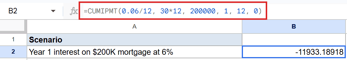
The cell lands at -$11,933.19 (full value -11933.18917911262). The negative sign means money out of your pocket. 0.06/12 is the monthly rate, 30*12 is 360 months, 200000 is the loan amount, periods 1 through 12 cover the first year, and the final 0 says payments are made at the end of each month.
Pro Tip: The interest you pay in year 1 of a mortgage is almost always the largest annual chunk because the loan balance is at its highest. As the principal drops, the interest portion of each payment drops with it.
Example 2: Total Interest Over the Full Life of a Car Loan
Set the first period to 1 and the last to the total number of months and CUMIPMT gives you the lifetime interest cost.
Below is the dataset, a single scenario in A2 covering a $25,000 car loan at 5 percent annual interest over 5 years.
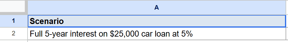
The goal is to add up every dollar of interest paid across all 60 monthly payments.
Here is the formula:
=CUMIPMT(0.05/12, 60, 25000, 1, 60, 0)
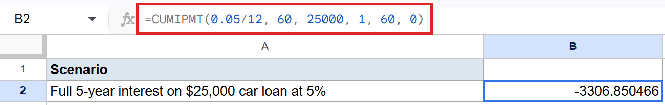
The cell lands at -$3,306.85 (full value -3306.850466016398). That is the true interest cost of the loan. The borrower pays back $25,000 in principal plus roughly $3,307 in interest, for a total of about $28,307 over 5 years.
This is a useful number for comparing financing offers. A loan with a lower monthly payment but a longer term often costs more in interest overall.
Example 3: Interest Paid in Year 2 of the Same Mortgage
Change the start and end periods to months 13 through 24 to see how year 2 compares.
Below is the dataset, a single scenario in A2, the same $200,000 mortgage at 6 percent over 30 years.
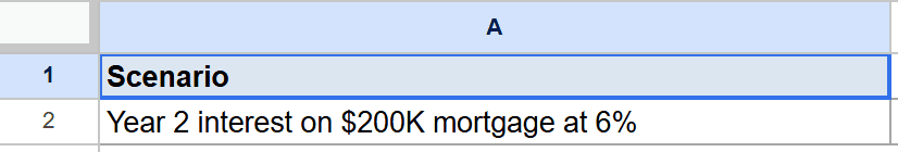
The goal is to total the interest for the second year of payments.
Here is the formula:
=CUMIPMT(0.06/12, 30*12, 200000, 13, 24, 0)
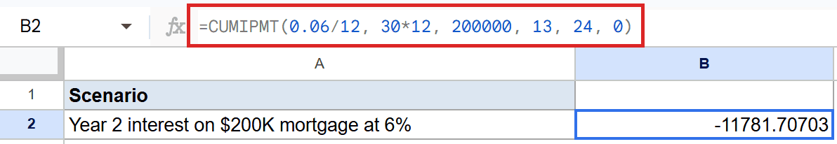
The cell lands at -$11,781.71 (full value -11781.707028398205). Notice this is a bit smaller than year 1’s interest. That is because some principal was paid down in year 1, so year 2 is computed against a slightly lower balance.
The gap is small at the start. Run CUMIPMT for year 25 or year 30 of the same loan and the difference is dramatic.
Example 4: CUMIPMT Driven by Parameter Cells
For a what-if loan sheet, point every CUMIPMT argument at a labeled input cell.
Below is the dataset, with rate in A2, periods in B2, present value in C2, start period in D2, and end period in E2.
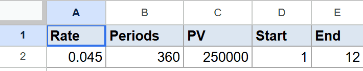
The goal is to compute the cumulative interest for the first year of a $250,000, 30-year mortgage at 4.5 percent.
Here is the formula:
=CUMIPMT(A2/12, B2, C2, D2, E2, 0)
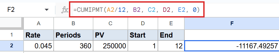
The cell lands at -$11,167.49 (full value -11167.492565565139). Notice A2/12 divides the annual rate by 12 right inside the formula. The input cell stays as the headline annual rate while the formula handles the monthly conversion.
Want to compare loans? Change the rate in A2 from 4.5 percent to 5.5 percent and watch the interest jump. Same for the term, the loan amount, or the period window.
Tips & Common Mistakes
- The result is always negative – interest is money paid out. If you want the positive dollar figure for a report, wrap CUMIPMT in ABS, or just flip the sign with a minus.
- Match the rate to the payment period – monthly payments need annual rate / 12 and total months for periods. Mixing an annual rate with monthly periods is the most common bug.
- First period is 1, not 0 – period 1 is the very first payment. Setting first_period to 0 throws a
#NUM!error.
That covers totaling interest for a year, a loan’s lifetime, or any custom window with CUMIPMT. Keep the rate matched to the payment period, remember the negative sign, and pair CUMIPMT with the SUM function or a parameter sheet when you need to compare multiple loans side by side.
List of All Google Sheets Functions
Related Google Sheets Functions / Articles: