
If you want to grab the smallest number from a list, but only from the rows that match one or more conditions, the MINIFS function in Google Sheets does it in a single call. You hand it the values to look at, a range to test, and the rule each row has to satisfy.
In this article, I’ll show you how to use MINIFS with a text label, a number threshold, two criteria at once, a date condition, and a wildcard match.
MINIFS Function Syntax in Google Sheets
The MINIFS function returns the minimum value from a range, considering only the rows that meet every criterion you pass.
=MINIFS(range, criteria_range1, criterion1, [criteria_range2, criterion2, ...])
- range is the column of numbers you want the minimum from.
- criteria_range1 is the column you test against the first rule.
- criterion1 is the rule a cell must meet, like “East”, “>10”, or “B*”.
- criteria_range2, criterion2, … are optional extra range and rule pairs. Add as many as you need; MINIFS only considers rows that satisfy every pair.
When to Use MINIFS Function
- Find the smallest value in rows that match a specific text label.
- Get the minimum value where another column clears a numeric threshold.
- Pull the smallest figure that satisfies two or more conditions at once.
- Find the lowest cost on or after a specific date.
- Use a wildcard to match a pattern of labels rather than an exact string.
Example 1: Find the Smallest Value Matching a Text Label
Let’s start with the most common case, finding the minimum for rows that match one label.
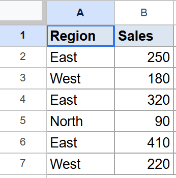
Below is the dataset. Column A has the region, with East repeating across multiple rows, and column B has the sales amount.
I want the smallest sales value among the East rows only.
Here is the formula:
=MINIFS(B2:B7, A2:A7, "East")
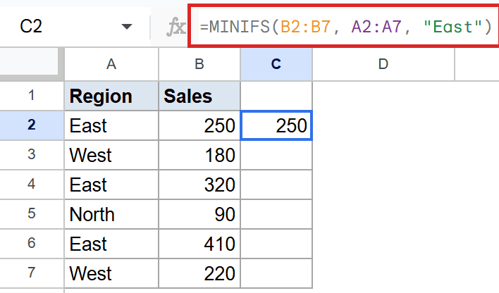
MINIFS looks down column A for “East”, then checks the matching sales in column B and returns the smallest of them. The East rows hold 250, 320, and 410, so the result is 250. The West and North rows are ignored entirely.
This is the conditional sibling of MAXIFS function. Where MAXIFS picks the largest value among the matching rows, MINIFS picks the smallest.
Example 2: Smallest Value That Beats a Number Threshold
The criterion can be a comparison, not just a text label.
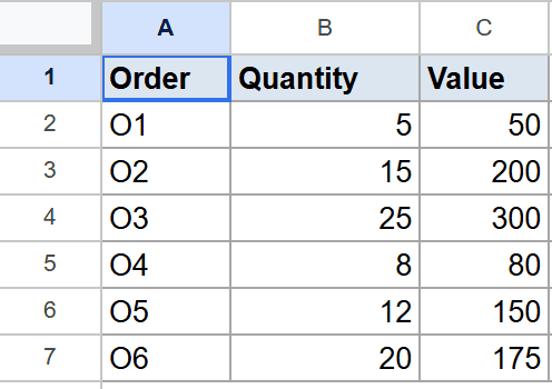
Below is the dataset. Column A has the order ID, column B has the quantity, and column C has the order value.
I want the smallest order value, but only for rows where the quantity is above ten.
Here is the formula:
=MINIFS(C2:C7, B2:B7, ">10")
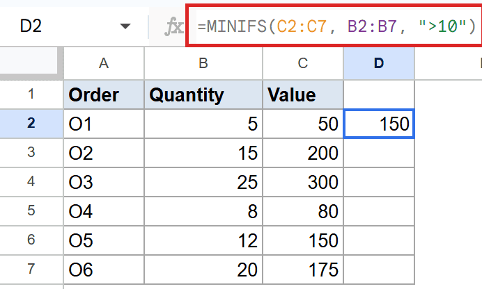
The criterion “>10” filters the rows down to the ones where quantity is greater than ten. That’s the rows with quantities 15, 25, 12, and 20. MINIFS then takes the smallest order value among those rows, which works out to 150.
Pro Tip: The operator and the number live inside one set of double quotes, like “>10”. If you want the threshold to come from a cell, concatenate it with the ampersand, like “>”&E1. Splitting the operator from the number without the ampersand breaks the formula.
Example 3: Smallest Value Matching Two Criteria At Once
You can pass more criteria pairs to narrow things down further.
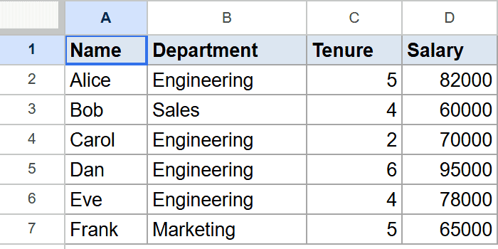
Below is the dataset. Column A has the employee name, column B has the department, column C has the tenure in years, and column D has the salary.
I want the smallest salary, but only for engineering employees with more than three years of tenure.
Here is the formula:
=MINIFS(D2:D7, B2:B7, "Engineering", C2:C7, ">3")
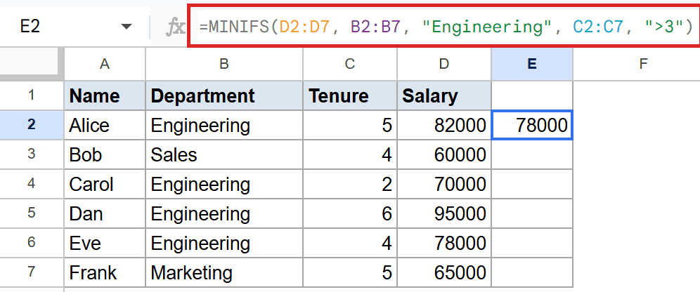
How this formula works:
- The first criterion pair narrows rows down to those where column B is “Engineering”. That’s Alice, Carol, Dan, and Eve.
- The second criterion pair further trims to rows where column C is above 3. Carol drops out (tenure 2), leaving Alice, Dan, and Eve.
- MINIFS then picks the smallest salary from those three, which is Eve’s at 78000.
Every criterion pair must use a range that’s the same size as the value range. If column D spans six rows, columns B and C must also span six rows.
Example 4: Smallest Value On Or After a Specific Date
You can compare against a date by building the criterion with the DATE function.
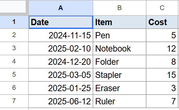
Below is the dataset. Column A has the transaction date, column B has the item, and column C has the cost.
I want the smallest cost from rows dated on or after the start of 2025.
Here is the formula:
=MINIFS(C2:C7, A2:A7, ">="&DATE(2025,1,1))
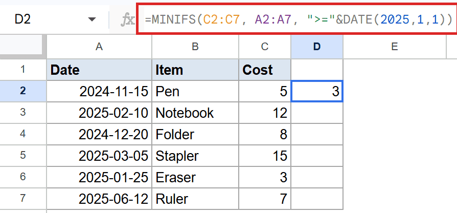
The expression “>=”&DATE(2025,1,1) builds the criterion at runtime. DATE returns the serial number for January 1, 2025, and the ampersand glues the “>=” operator to that number, producing a valid criterion string.
Four rows fall on or after that date. Their costs are 12, 15, 3, and 7, so MINIFS returns the smallest, which works out to 3.
Pro Tip: For date criteria, always build the date with DATE(year, month, day) instead of typing it as text. Text dates like “2025-01-01” can be parsed inconsistently across locales. DATE always returns the correct serial number.
Example 5: Smallest Value With a Wildcard Text Match
You can match a pattern of labels with an asterisk wildcard.
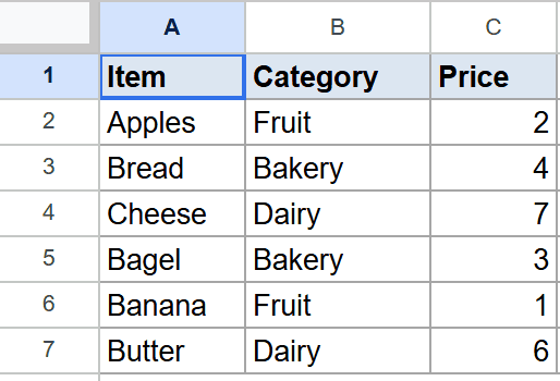
Below is the dataset. Column A has the item, column B has the category, and column C has the price.
I want the smallest price among items in any category whose name starts with the letter B.
Here is the formula:
=MINIFS(C2:C7, B2:B7, "B*")
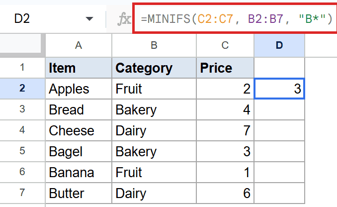
The asterisk in “B*” stands for any characters that follow, so it matches any category that starts with B. In this dataset, only Bakery qualifies, since none of the others start with B. The Bakery rows hold prices 4 and 3, so the result is 3.
Use a question mark instead of an asterisk when you want to match exactly one character rather than any number of them.
Tips & Common Mistakes
- Wrap operators and patterns in double quotes. Conditions like “>10”, “<>100”, “B*”, and even plain text like “East” must sit inside quotes, or the formula won’t parse. Cell references stay outside the quotes and join in with the ampersand.
- Every range has to be the same size. The value range, every criteria range, they all need to span the same number of rows. If they don’t line up, MINIFS returns a #VALUE! error instead of a number.
- Empty matches return zero, not an error. If no row satisfies the criteria, MINIFS returns 0. That can look like a valid minimum if your data legitimately contains zero, so wrap MINIFS in an IF function test if you want to display “No match” instead.
MINIFS is the cleanest way to grab the smallest value from filtered rows. No helper columns, no sort, no array formula gymnastics.
You’ve now seen it on a text label, a number threshold, two conditions at once, a date comparison, and a wildcard. Pick the criterion shape that matches your data and MINIFS handles the rest.
List of All Google Sheets Functions
Related Google Sheets Functions / Articles: