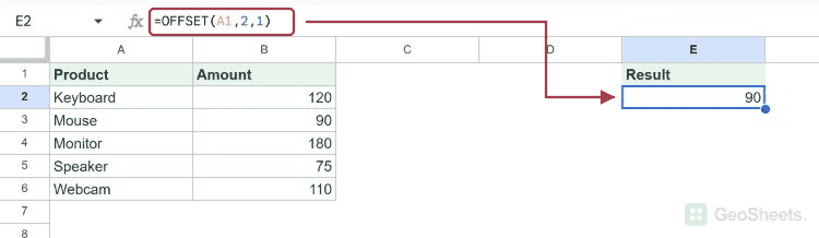
If you want to grab a value or a range that sits a certain number of rows and columns away from a starting cell, the OFFSET function in Google Sheets is built for exactly that.
You give it an anchor cell and tell it how far to move, and it hands back the reference at that spot. In this article, I’ll walk you through five examples, from pulling a single cell to returning a whole range that other functions can use.
OFFSET Function Syntax in Google Sheets
OFFSET starts at an anchor cell and shifts away from it by a set number of rows and columns.
=OFFSET(cell_reference, offset_rows, offset_columns, [height], [width])
cell_reference: the anchor cell or range you measure from.offset_rows: how many rows to move. Positive moves down, negative moves up, 0 stays put.offset_columns: how many columns to move. Positive moves right, negative moves left, 0 stays put.height(optional): how many rows tall the returned range should be.width(optional): how many columns wide the returned range should be.
If you leave out height and width, OFFSET returns a single cell. Supply them and it returns a range of that size, which can spill into the cells below and to the right.
When to Use OFFSET Function
- Pull a value that sits a fixed distance from a known anchor cell.
- Sum or average a block of cells without typing out the full range.
- Return a dynamic range whose size changes as your data grows.
- Combine with MATCH to fetch a value next to a looked-up item.
- Build a moving window that always points at the last few rows of a list.
Example 1: Pull a single cell from an anchor
Let’s start with the simplest case, moving a fixed number of rows and columns from one cell.
Below is the dataset with a small grid of values in A1:C3, where row 1 holds headers and the rows below hold numbers.

The goal is to grab the value that sits two rows down and one column right of cell A1.
Here is the formula:
=OFFSET(A1,2,1)

Starting at A1, OFFSET moves down two rows and right one column, landing on cell B3. The value there is 0.8, so that is what the formula returns.
Think of it as counting from the anchor. Rows count downward, columns count rightward, and either count can be zero if you don’t want to move in that direction.
Pro Tip: OFFSET returns a reference, not just a value, so it behaves like the cell it lands on. If you want the text address of that cell instead, the [ADDRESS](https://geosheets.com/google-sheets-function/address/) function builds a reference string from row and column numbers.
Example 2: Sum a range built with OFFSET
OFFSET can return a whole range, and you can hand that range straight to SUM. Here we add up a column of values starting one row below the header.
Below is the dataset with a header in A1 and five monthly amounts in A2:A6.

The goal is to total the five amounts without typing the range A2:A6 directly.
Here is the formula:
=SUM(OFFSET(A1,1,0,5,1))

How this formula works:
- Starting at A1, OFFSET moves down one row and zero columns, so it lands on A2.
- The height of 5 and width of 1 make it return the 5-row, 1-column range A2:A6.
- SUM then adds those five values together.
The total comes out to 1000. Because the range is built from a count rather than typed out, you can change the height to cover more or fewer rows.
Example 3: Return a range that spills
This is where OFFSET shows off. With a height and width, it returns a full range that spills across multiple cells.
Below is the dataset with a Name and Score table in A1:C3.

The goal is to copy the first three rows and first two columns of the table into a new spot.
Here is the formula:
=OFFSET(A1,0,0,3,2)

How this formula works:
- The row and column offsets are both 0, so OFFSET stays anchored at A1.
- The height of 3 and width of 2 tell it to return a 3-row, 2-column block.
- That block is the range A1:B3, which spills out of the formula cell.
The result spills into a 3 by 2 grid showing the headers Name and Score, then Alice with 87, and Bob with 72. Only the top-left cell holds the formula. The rest fill in automatically.
Example 4: Average the last three rows of a list
OFFSET shines when the range needs to move as data grows. Here we always average the last three entries, even after new rows are added.
Below is the dataset with a header in A1 and a growing column of daily values in A2 downward.

The goal is to average the most recent three values without updating the formula by hand.
Here is the formula:
=AVERAGE(OFFSET(A1,COUNT(A2:A100)-2,0,3,1))

How this formula works:
- COUNT tallies how many numbers sit in A2:A100. Subtracting 2 lands the offset on the third-from-last value.
- OFFSET then returns a 3-row, 1-column range starting there, which is the last three entries.
- AVERAGE works out the mean of those three values.
The result is 50. Add a new value to the bottom of the column and the window slides down on its own, always covering the latest three rows.
Example 5: Fetch a value next to a matched item
Pair OFFSET with MATCH and you get a flexible lookup that finds a row first, then steps sideways to the value you want.
Below is the dataset with product names in column A, their prices in column B, and the product you want to find typed into C2.

The goal is to return the price of the product named in C2.
Here is the formula:
=OFFSET(A1,MATCH(C2,A2:A7,0),1)

How this formula works:
- The MATCH function finds the position of the product from C2 within the list A2:A7.
- That position becomes the row offset, so OFFSET steps down from A1 to the matching product’s row.
- The column offset of 1 then moves one column right, landing on the price in column B.
The formula returns 140 for the matched product. Swap the name in C2 and the price updates to match.
Pro Tip: This OFFSET and MATCH combo works as a lookup, but for everyday matching a dedicated lookup like VLOOKUP or the [HLOOKUP](https://geosheets.com/google-sheets-function/hlookup/) function is easier to read. Save the OFFSET approach for when you need a moving or resizable range.
Tips & Common Mistakes
- OFFSET is volatile. It recalculates on every change anywhere in the sheet, not just when its inputs change. A few are fine, but hundreds of OFFSET formulas can slow a large workbook down.
- Watch for out-of-bounds offsets. If the row or column offset pushes past the edge of the sheet, OFFSET returns a
#REF!error. Double-check that your counts keep the result inside the grid. - Offsets can be zero or negative. Zero rows and zero columns keeps you on the anchor. Negative values move up or left, which is handy but easy to forget when you’re counting only downward and rightward.
OFFSET is a flexible way to point at a cell or a range a set distance from an anchor, and it really pays off when that range needs to resize or move as your data changes. Just keep an eye on its volatility and stay inside the sheet’s bounds.
List of All Google Sheets Functions
Related Google Sheets Functions / Articles: